R2D - Liquefaction
Introduction
This page describes basic concepts of geospatial liquefaction hazard modeling withing the umbrella of SimCenter tools.
Problem Description
Coseismic soil liquefaction is a phenomenon in which the strength and stiffness of a soil is reduced by earthquake shaking. Resilient communities and infrastructure networks, like lifelines or transportation systems, must be built to withstand and respond to hazards posed by coseismic soil liquefaction. Ideally, these predictions could be made:
quickly, in near-real-time after an event;
at high resolution, consistent with the scale of individual assets; and
at map-scale, across the regional extent affected by large earthquakes.
Common liquefaction models in practice require in-situ testing which cannot be continuously performed across large areas, thus presenting the need for “geospatial” liquefaction models. Prior tests of such models (e.g., [ZBT17]) have shown both promising potential and severe shortcomings in predicting subsurface conditions with few geospatial predictors. There is a need to advance geospatial liquefaction modeling by integrating geotechnical data, liquefaction mechanics, artificial intelligence (AI), and many geospatial predictor variables to provide reliable regional liquefaction predictions for any earthquake event. When integrated with regional hazard assessment capabilities, geospatial liquefcation models will provide value throughout the life of infrastructure projects - from initial desk studies to refined project-specific hazard analyses - and will unlock insights beyond conventional practice, with opportunity to:
prescribe event-specific emergency response and evacuation routes immediately after an earthquake,
evaluate network reliability and infrastructure network resiliency using structural databases or other asset inventories, and
understand the impacts of earthquake events of vulnerable communities using population demographic data.
Solution Strategy
The state-of-practice geospatial liquefaction model is the [RB20] model (updated version of the [ZBT17] model), which uses logistic regression to predict probability of liquefaction based on five (5) geospatial variables and trained on a database of liquefaction case histories.
In this problem, another modeling solution strategy is proposed, according to [SGM24]. The [SGM24] approach parses the problem into that which is empirical and best predicted by AI (the relationship between geospatial variables and subsurface traits) and that which is best predicted by mechanics (liquefaction response, conditioned on those traits). In this approach, the subsurface traits are characterized at point locations using available cone penetration testing (CPT) data. The liquefaction response at each CPT location is computed across a range of magnitude-scale peak ground accelerations (PGAM7.5) using state-of-practice liquefaction manifestation models (e.g., liquefaction potential index, LPI), thereby retaining the knowledge of liquefaction mechanics developed over the last 50+ years. The relationship between manifestation index and PGAM7.5 is represented as a functional form (Eqn 1) with two curve-fitting parameters: A and B (Fig 1). Therefore, the liquefaction response (i.e., A and B) at each CPT location becomes target variables of supervised learning AI models.
Eqn 1. Manifestation index as a function of A, B, and PGAM7.5.
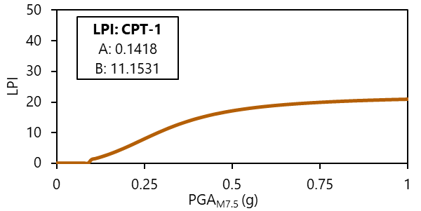
Fig 1. Example manifestation curve of LPI vs. PGAM7.5 for a single CPT.
The AI model is trained to predict liquefaction response using a set of 37 geospatial predictor variables that serve as proxies for liquefaction. These predictor variables include metrics of surface topography and roughness, distance to and elevation above water bodies, and information about geology, geomorphology, and hydrology. By applying the trained AI model to these predictor datasets, the A and B parameters are predicted geospatially at 100-meter resolution. A crucial step in this approach is geostatistically updating the AI predictions via regression kriging near field measurements. The effect is that predictions near known subsurface conditions have lower model uncertainty, while predictions farther away rely on the AI model and have higher uncertainty. This method effectively pre-computes liquefaction response for all possible ground motions based on AI-predicted subsurface conditions. These predictions are stored as mapped parameters, ready for use with specific earthquake data, such as a PGAM7.5 raster in R2D.
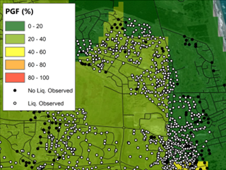
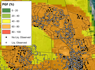
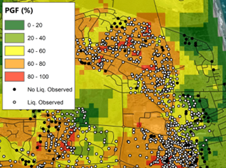
Model predictions were then tested against the leading geospatial model [RB20] in three case-history events using receiver operating characteristic and area under the curve analyses (Fig 2). The [SGM24] AI model (before kriging) performed significantly better than [RB20] and was further improved by kriging (Fig 3).
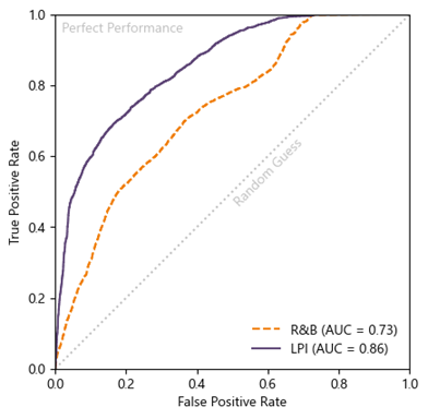
Fig 2. Receiver operator characteristic curves and area under the curve (AUC) analyses comparing [RB20] (“R&B”), and the [SGM24] before regression kriging (“LPI”).
(a)
(b)
(c)
Fig 3. Comparison between (a) Rashidian & Baise (2020), and this model (b) before and (c) after regression kriging for the Feb. 2011 M6.1 Christchurch event.
SimCenter Tool Used
The presented problem can be solved using SimCenter’s Regional Resilience Determination R2D Tool. A substantially complete description of the tool is provided in the R2D Documentation.
The updated [ZBT17] model ([RB20]) is implemented in the R2D tool (version 4.2.0), whereas the [SGM24] model is not yet implemented in the R2D tool. In this project, the [SGM24] model was implemented in the R2D tool using the applications.py file.
The workflow for the [ZBT17] model in the Earthquake Event Generator tool in R2D is as follows:
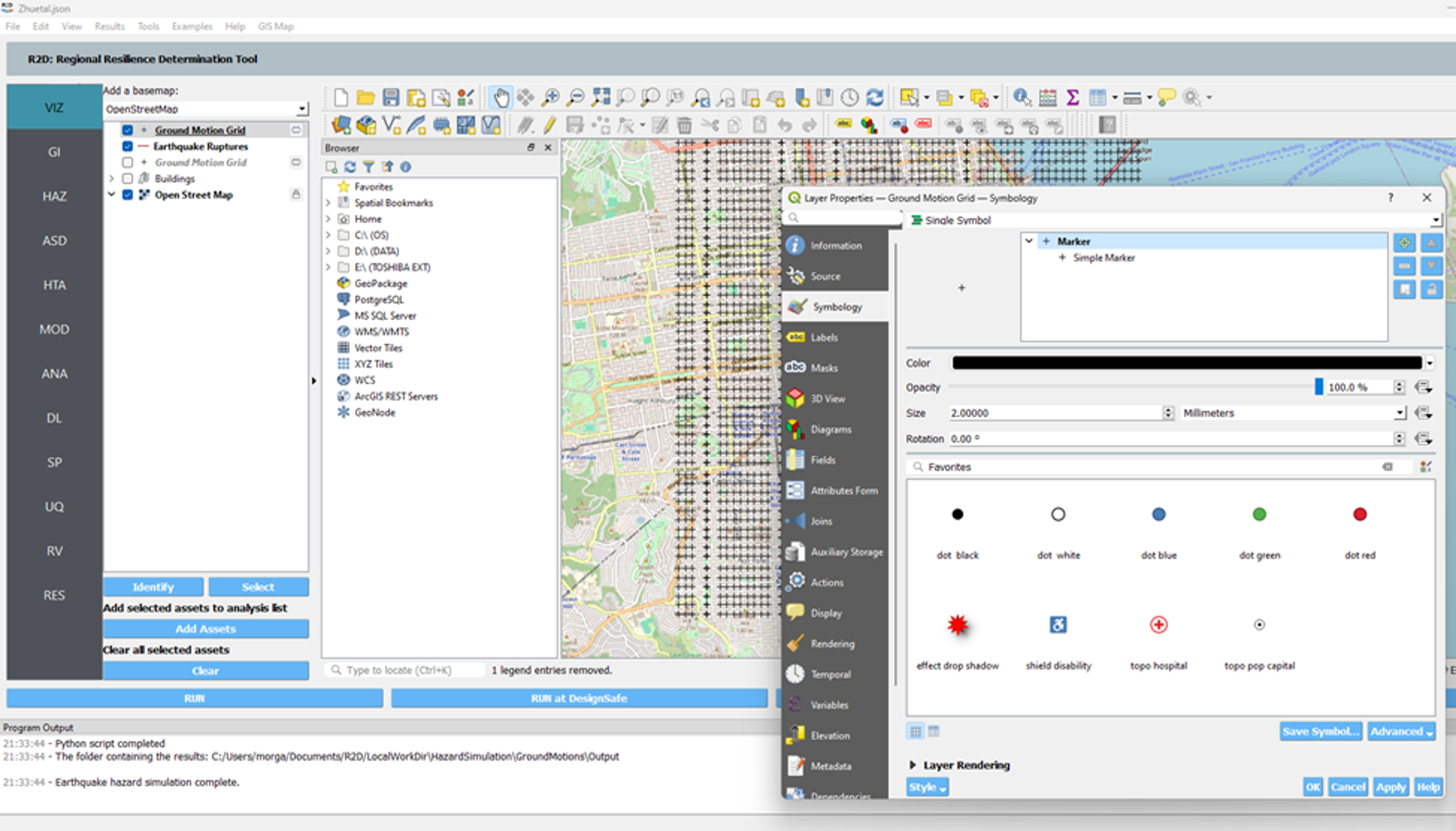
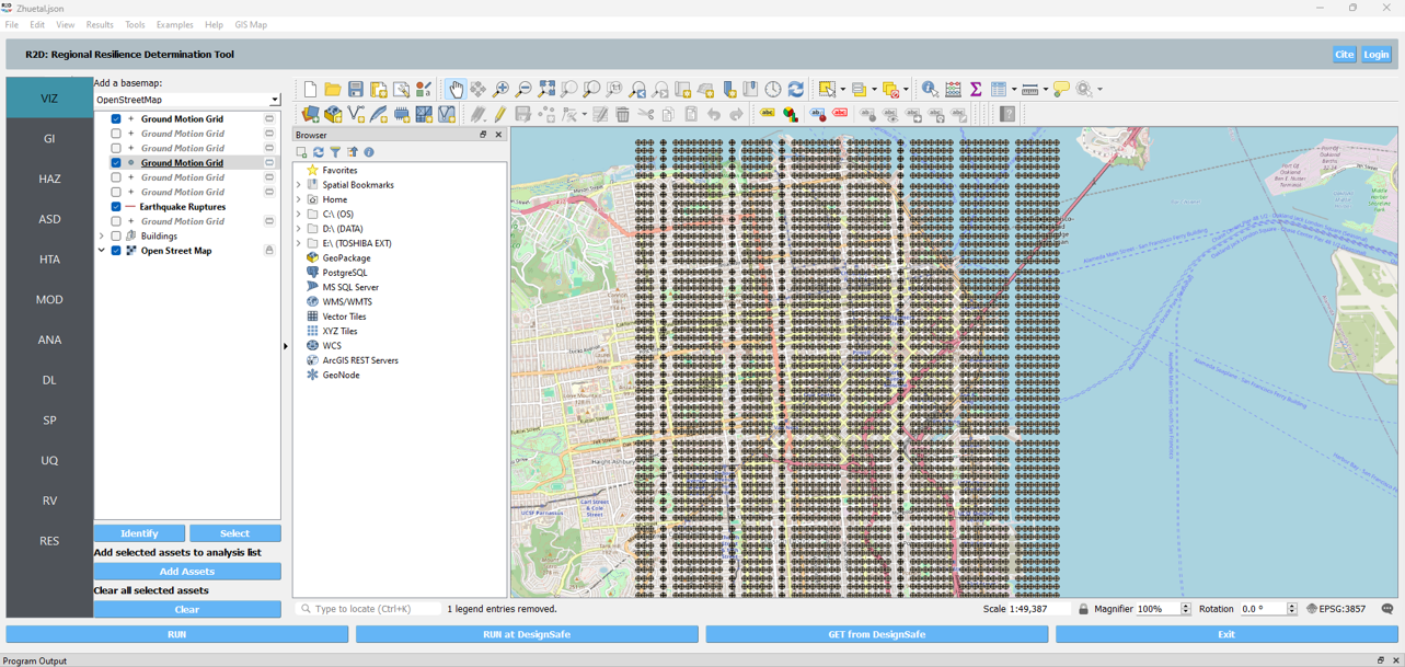
1. Define Analysis Grid: Define the analysis grid for the study area. Here, an area of downtown San Francisco is selected for the analysis. The grid is defined with a resolution of approximately 100 meters, the true model resolution of the [SGM24] model.

2. Forecast Rupture Scenarios: Large events (>M7) are forecasted for the study area to demonstrate the model performance under extreme conditions.
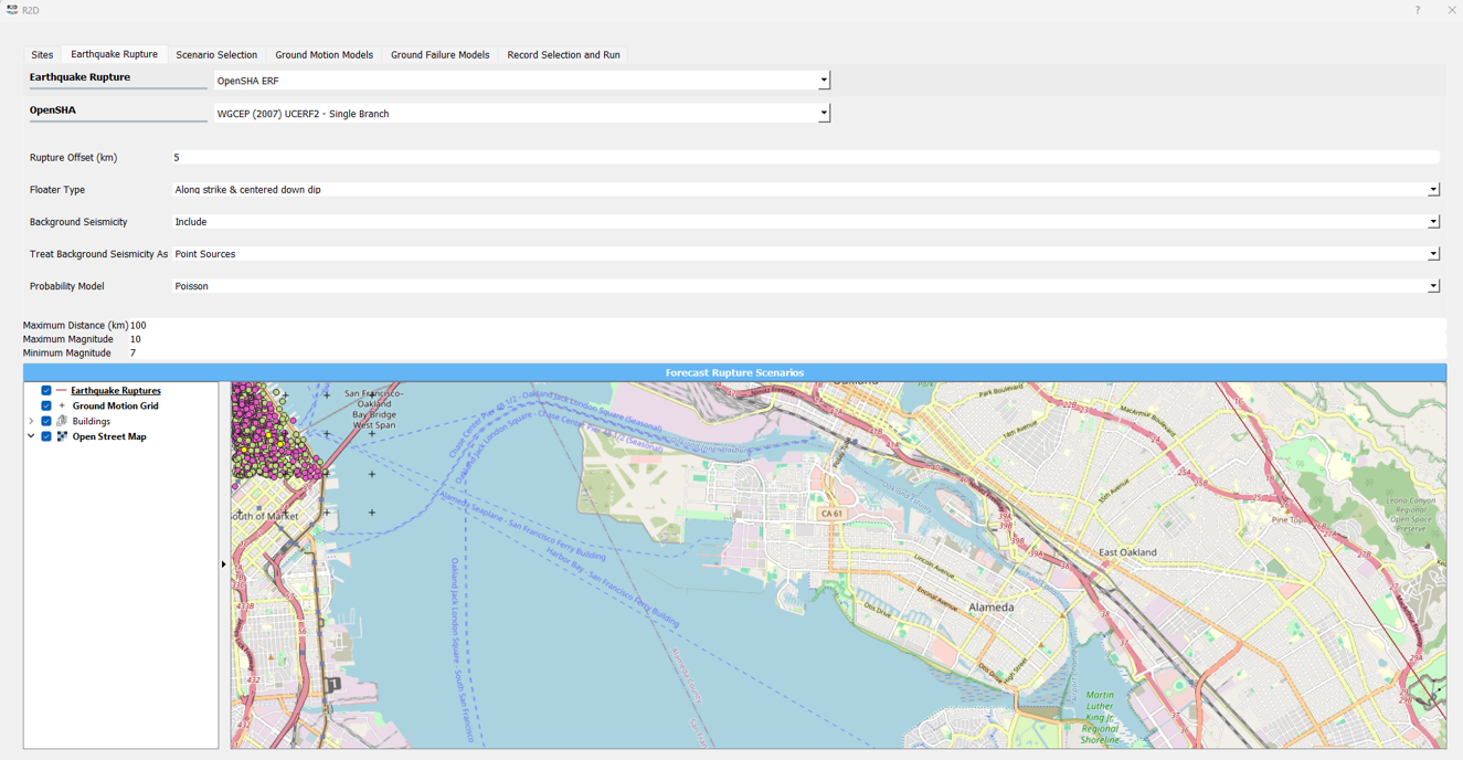
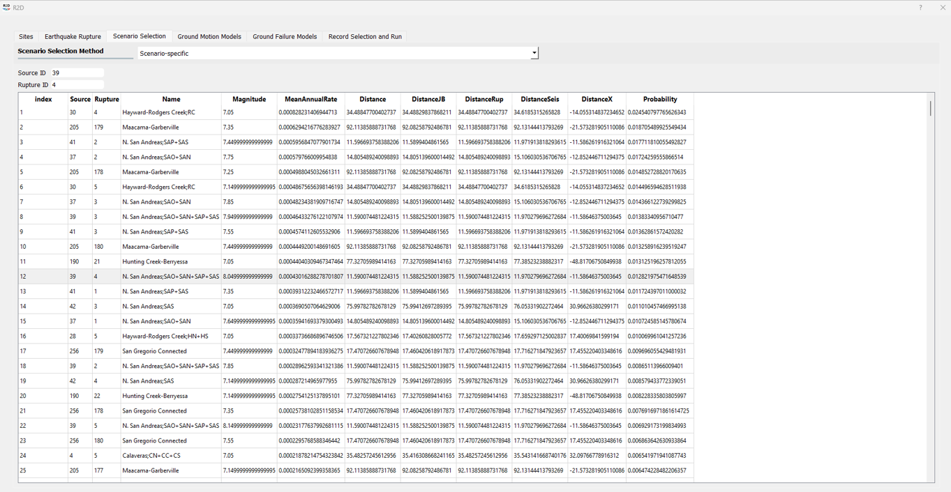
3. Select Earthquake Event: Select an earthquake event scenario. Here, the M8 N. San Andreas rupture event scenario is selected.
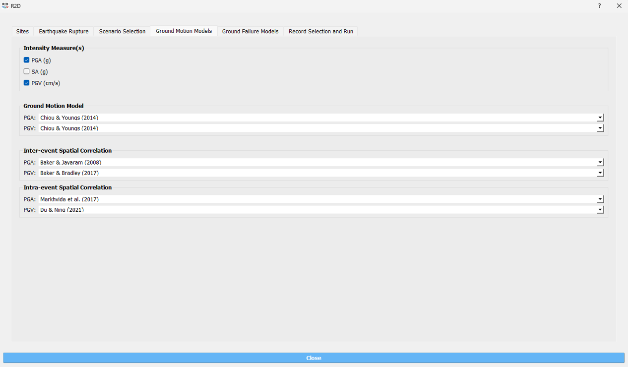
4. Select Intensity Measures: PGA and PGV are selected as the intensity measures for the analysis, both required for the [ZBT17] model.
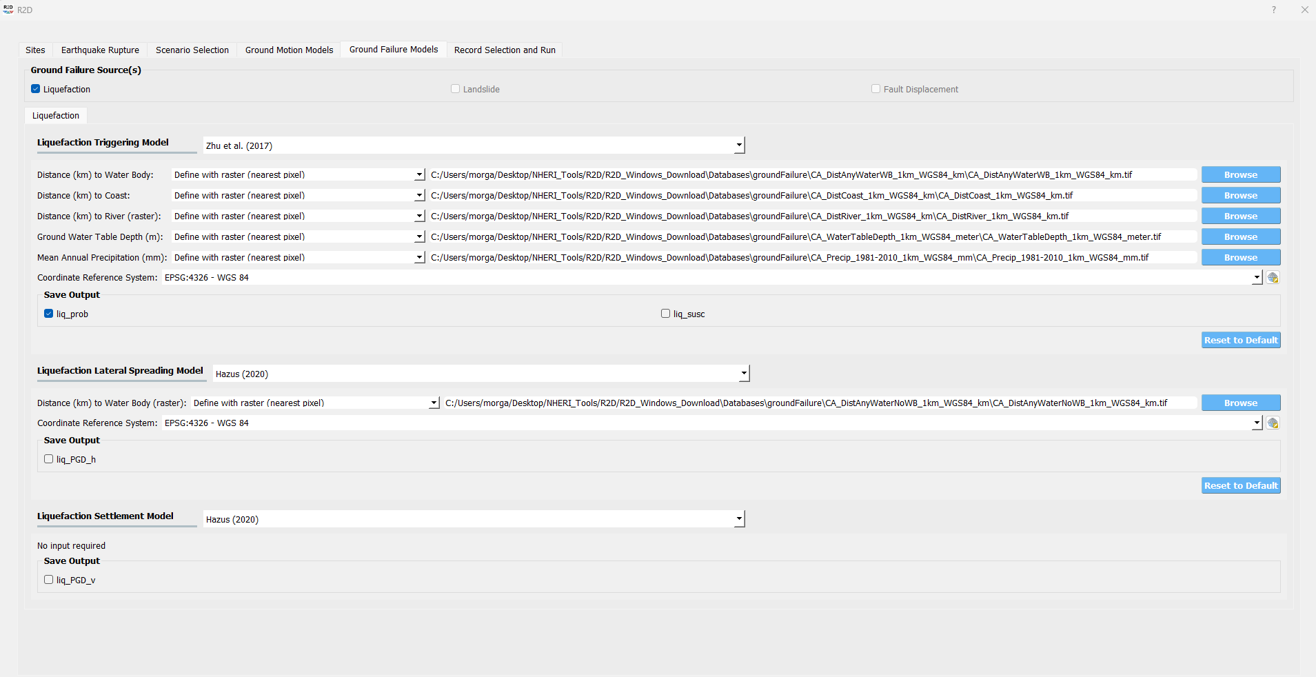
5. Select Ground Failure Model: Select the ground failure model. Here, the [ZBT17] model is selected.
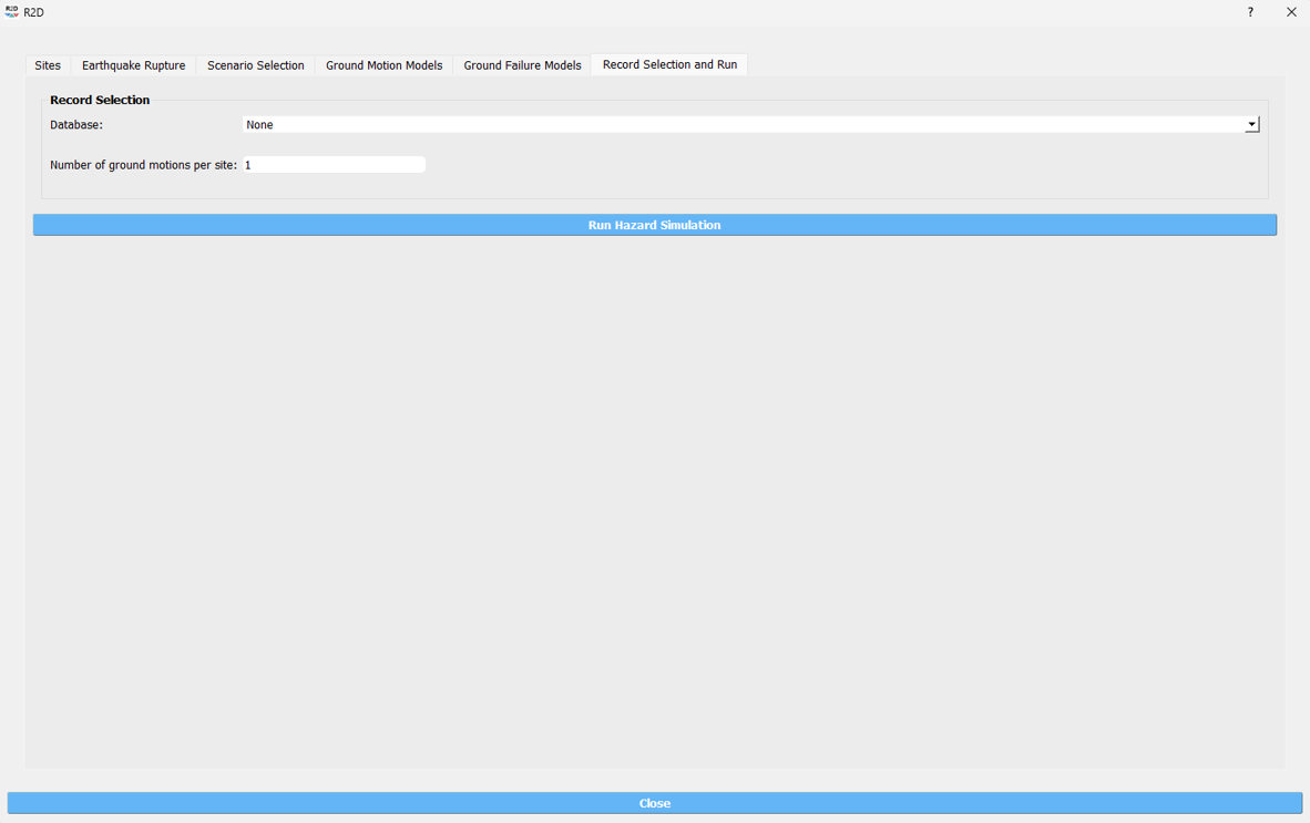
6. Run Hazard Simulation.
7. View Results
Example Application
This example demonstrates the application of the [ZBT17] liquefaction-induced ground failure model (really the [RB20] model) currently implemented in R2D, and the implementation of the next-generation [SGM24] model described in the Solution Strategy.
Note
In R2D, ground failure models are considered intermediate results that are accessible only through the Earthquake Event Generator tool, and they cannot be executed within the damage and loss assessment tools. Future development in R2D should consider (1) implementing ground failure models with other earthquake hazard source options (e.g., Shakemap Earthquake Scenario), (2) extending the implementation of the ground failure modeling beyond California, and (3) incorporating ground failure models into the damage and loss assessment tools.
Note
The implementation of the [ZBT17] and [SGM24] models in the Earthquake Event Generator tool employs grid sampling of the geospatial parameters, which is not the most efficient method for large-scale applications. Future development in R2D should consider implementing the models as raster-based models for more efficient, higher resolution, spatially continuous predictions in accordance with the model development.
Zhu et al. (2017)
CODE
The following code snippet shows the implementation of the [ZBT17] model in the R2D tool using the applications.py file.
Click to expand the full ZhuEtal2017 code
  1# Zhu et al. (2017) code
  2-----------------------------------------------------------
  3class ZhuEtal2017(Liquefaction):
  4    """
  5    A map-based procedure to quantify liquefaction at a given location using logistic models by Zhu et al. (2017). Two models are provided:
  6
  7    1. For distance to coast < cutoff, **prob_liq** = f(**pgv**, **vs30**, **precip**, **dist_coast**, **dist_river**)
  8    2. For distance to coast >= cutoff, **prob_liq** = f(**pgv**, **vs30**, **precip**, **dist_coast**, **dist_river**, **gw_depth**)
  9
 10    Parameters
 11    ----------
 12    From upstream PBEE:
 13    pgv: float, np.ndarray or list
 14        [cm/s] peak ground velocity
 15    mag: float, np.ndarray or list
 16        moment magnitude
 17    pga: float, np.ndarray or list
 18        [g] peak ground acceleration, only to check threshold where prob_liq(pga<0.1g)=0
 19    stations: list
 20        a list of dict containing the site infomation. Keys in the dict are 'ID',
 21        'lon', 'lat', 'vs30', 'z1pt0', 'z2pt5', 'vsInferred', 'rRup', 'rJB', 'rX'
 22
 23    Geotechnical/geologic:
 24    vs30: float, np.ndarray or list
 25        [m/s] time-averaged shear wave velocity in the upper 30-meters
 26    precip: float, np.ndarray or list
 27        [mm] mean annual precipitation
 28    dist_coast: float, np.ndarray or list
 29        [km] distance to nearest coast
 30    dist_river: float, np.ndarray or list
 31        [km] distance to nearest river
 32    dist_water: float, np.ndarray or list
 33        [km] distance to nearest river, lake, or coast
 34    gw_depth: float, np.ndarray or list
 35        [m] groundwater table depth
 36
 37    Fixed:
 38    # dist_water_cutoff: float, optional
 39    #     [km] distance to water cutoff for switching between global and coastal model, default = 20 km
 40
 41    Returns
 42    -------
 43    prob_liq : float, np.ndarray
 44        probability for liquefaciton
 45    liq_susc_val : str, np.ndarray
 46        liquefaction susceptibility category value
 47
 48    References
 49    ----------
 50    .. [1] Zhu, J., Baise, L.G., and Thompson, E.M., 2017, An Updated Geospatial Liquefaction Model for Global Application, Bulletin of the Seismological Society of America, vol. 107, no. 3, pp. 1365-1385.
 51
 52    """
 53    def __init__(self, parameters, stations) -> None:
 54        self.stations = stations
 55        self.parameters = parameters
 56        self.dist_to_water = None #(km)
 57        self.dist_to_river = None #(km)
 58        self.dist_to_coast = None #(km)
 59        self.gw_depth = None #(m)
 60        self.precip = None # (mm)
 61        self.vs30 = None #(m/s)
 62        self.interpolate_spatial_parameters(parameters)
 63
 64    def interpolate_spatial_parameters(self, parameters):
 65        # site coordinate in CRS 4326
 66        lat_station = [site['lat'] for site in self.stations]
 67        lon_station = [site['lon'] for site in self.stations]
 68        # dist_to_water
 69        if parameters["DistWater"] == "Defined (\"distWater\") in Site File (.csv)":
 70            self.dist_to_water = np.array([site['distWater'] for site in self.stations])
 71        else:
 72            self.dist_to_water = sampleRaster(parameters["DistWater"], parameters["inputCRS"],\
 73                    lon_station, lat_station)
 74        # dist_to_river
 75        if parameters["DistRiver"] == "Defined (\"distRiver\") in Site File (.csv)":
 76            self.dist_to_river = np.array([site['distRiver'] for site in self.stations])
 77        else:
 78            self.dist_to_river = sampleRaster(parameters["DistRiver"], parameters["inputCRS"],\
 79                    lon_station, lat_station)
 80        # dist_to_coast
 81        if parameters["DistCoast"] == "Defined (\"distCoast\") in Site File (.csv)":
 82            self.dist_to_coast = np.array([site['distCoast'] for site in self.stations])
 83        else:
 84            self.dist_to_coast = sampleRaster(parameters["DistCoast"], parameters["inputCRS"],\
 85                    lon_station, lat_station)
 86        # gw_water
 87        if parameters["GwDepth"] == "Defined (\"gwDepth\") in Site File (.csv)":
 88            self.gw_depth = np.array([site['gwDepth'] for site in self.stations])
 89        else:
 90            self.gw_depth = sampleRaster(parameters["GwDepth"], parameters["inputCRS"],\
 91                    lon_station, lat_station)
 92        # precipitation
 93        if parameters["Precipitation"] == "Defined (\"precipitation\") in Site File (.csv)":
 94            self.precip = np.array([site['precipitation'] for site in self.stations])
 95        else:
 96            self.precip = sampleRaster(parameters["Precipitation"], parameters["inputCRS"],\
 97                    lon_station, lat_station)
 98        self.vs30 = np.array([site['vs30'] for site in self.stations])
 99        print("Sampling finished")
100
101    def run(self, ln_im_data, eq_data, im_list, output_keys, additional_output_keys):
102        if ('PGA' in im_list) and ('PGV' in im_list):
103            num_stations = len(self.stations)
104            num_scenarios = len(eq_data)
105            PGV_col_id = [i for i, x in enumerate(im_list) if x == 'PGV'][0]
106            PGA_col_id = [i for i, x in enumerate(im_list) if x == 'PGA'][0]
107            for scenario_id in range(num_scenarios):
108                num_rlzs = ln_im_data[scenario_id].shape[2]
109                im_data_scen = np.zeros([num_stations,\
110                                    len(im_list)+len(output_keys), num_rlzs])
111                im_data_scen[:,0:len(im_list),:] = ln_im_data[scenario_id]
112                for rlz_id in range(num_rlzs):
113                    pgv = np.exp(ln_im_data[scenario_id][:,PGV_col_id,rlz_id])
114                    pga = np.exp(ln_im_data[scenario_id][:,PGA_col_id,rlz_id])
115                    mag = float(eq_data[scenario_id][0])
116                    model_output = self.model(pgv, pga, mag)
117                    for i, key in enumerate(output_keys):
118                        im_data_scen[:,len(im_list)+i,rlz_id] = model_output[key]
119                ln_im_data[scenario_id] = im_data_scen
120            im_list = im_list + output_keys
121            additional_output = dict()
122            for key in additional_output_keys:
123                item = getattr(self, key, None)
124                if item is None:
125                    warnings.warn(f"Additional output {key} is not avaliable in the liquefaction trigging model 'ZhuEtal2017'.")
126                else:
127                    additional_output.update({key:item})
128        else:
129            sys.exit(f"At least one of 'PGA' and 'PGV' is missing in the selected intensity measures and the liquefaction trigging model 'ZhuEtal2017' can not be computed.")
130            # print(f"At least one of 'PGA' and 'PGV' is missing in the selected intensity measures and the liquefaction trigging model 'ZhuEtal2017' can not be computed."\
131            #       , file=sys.stderr)
132            # sys.stderr.write("test")
133            # sys.exit(-1)
134        return ln_im_data, eq_data, im_list, additional_output
135
136    def model(self, pgv, pga, mag):
137        """Model"""
138        # zero prob_liq
139        zero_prob_liq = 1e-5 # decimal
140
141        # distance cutoff for model
142        model_transition = 20 # km
143
144        # initialize arrays
145        x_logistic = np.empty(pgv.shape)
146        prob_liq = np.empty(pgv.shape)
147        liq_susc_val = np.ones(pgv.shape)*-99
148        liq_susc = np.empty(pgv.shape, dtype=int)
149
150        # magnitude correction, from Baise & Rashidian (2020) and Allstadt et al. (2022)
151        pgv_mag = pgv/(1+np.exp(-2*(mag-6)))
152        pga_mag = pga/(10**2.24/mag**2.56)
153
154        # find where dist_water <= cutoff for model of 20 km
155        # coastal model
156        ind_coastal = self.dist_to_water<=model_transition
157        # global model
158        # ind_global = list(set(list(range(pgv.shape[0]))).difference(set(ind_coastal)))
159        ind_global = ~(self.dist_to_water<=model_transition)
160
161        # set cap of precip to 1700 mm
162        self.precip[self.precip>1700] = 1700
163
164        # x = b0 + b1*var1 + ...
165        # if len(ind_global) > 0:
166        # liquefaction susceptbility value, disregard pgv term
167        liq_susc_val[ind_global] = \
168            8.801 + \
169            -1.918   * np.log(self.vs30[ind_global]) + \
170            5.408e-4 * self.precip[ind_global] + \
171            -0.2054  * self.dist_to_water[ind_global] + \
172            -0.0333  * self.gw_depth[ind_global]
173        # liquefaction susceptbility value, disregard pgv term
174        liq_susc_val[ind_coastal] = \
175            12.435 + \
176            -2.615   * np.log(self.vs30[ind_coastal]) + \
177            5.556e-4 * self.precip[ind_coastal] + \
178            -0.0287  * np.sqrt(self.dist_to_coast[ind_coastal]) + \
179            0.0666   * self.dist_to_river[ind_coastal] + \
180            -0.0369  * self.dist_to_river[ind_coastal]*np.sqrt(self.dist_to_coast[ind_coastal])
181        # catch nan values
182        liq_susc_val[np.isnan(liq_susc_val)] = -99.
183        # x-term for logistic model = liq susc val + pgv term
184        x_logistic[ind_global] = liq_susc_val[ind_global] + 0.334*np.log(pgv_mag[ind_global])
185        # x-term for logistic model = liq susc val + pgv term
186        x_logistic[ind_coastal] = liq_susc_val[ind_coastal] + 0.301*np.log(pgv_mag[ind_coastal])
187
188        # probability of liquefaction
189        prob_liq = 1/(1+np.exp(-x_logistic)) # decimal
190        prob_liq = np.maximum(prob_liq,zero_prob_liq) # set prob to > "0" to avoid 0% in log
191
192        # for pgv_mag < 3 cm/s, set prob to "0"
193        prob_liq[pgv_mag<3] = zero_prob_liq
194        # for pga_mag < 0.1 g, set prob to "0"
195        prob_liq[pga_mag<0.1] = zero_prob_liq
196        # for vs30 > 620 m/s, set prob to "0"
197        prob_liq[self.vs30>620] = zero_prob_liq
198
199        # calculate sigma_mu
200        sigma_mu = (np.exp(0.25)-1) * prob_liq
201
202        # determine liquefaction susceptibility category
203        liq_susc[liq_susc_val>-1.15]  = liq_susc_enum['very_high'].value
204        liq_susc[liq_susc_val<=-1.15] = liq_susc_enum['high'].value
205        liq_susc[liq_susc_val<=-1.95] = liq_susc_enum['moderate'].value
206        liq_susc[liq_susc_val<=-3.15] = liq_susc_enum['low'].value
207        liq_susc[liq_susc_val<=-3.20] = liq_susc_enum['very_low'].value
208        liq_susc[liq_susc_val<=-38.1] = liq_susc_enum['none'].value
209
210        # liq_susc[prob_liq==zero_prob_liq] = 'none'
211
212        return {"liq_prob":prob_liq, "liq_susc":liq_susc}
RESULTS
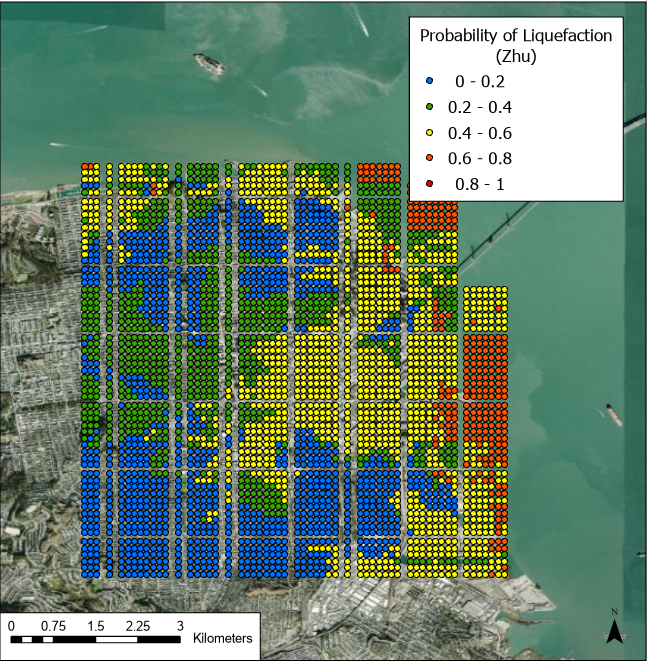
Fig 4. Results of the Zhu et al. (2017) model for probability of liquefaction given the selected M8 N. San Andreas rupture event scenario.
Sanger et al. (2024)
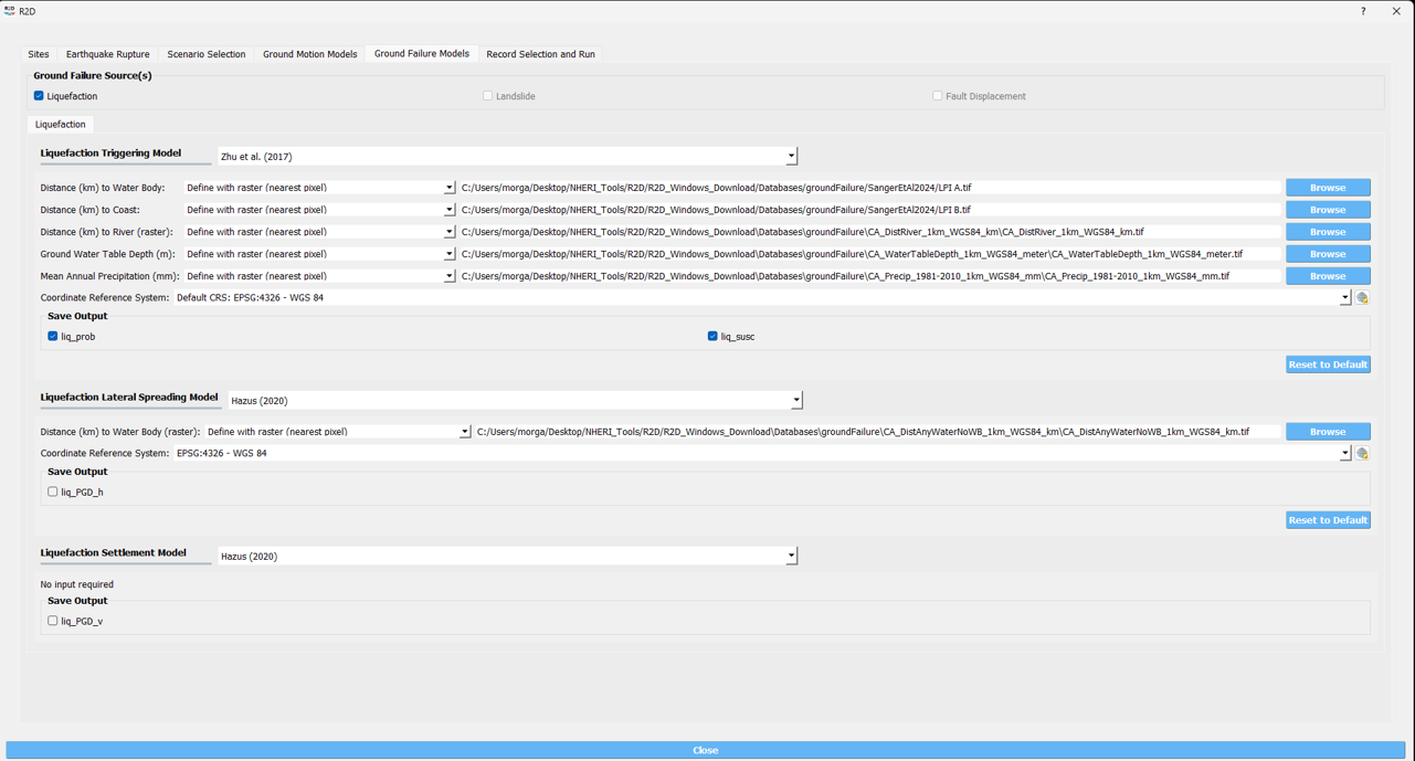
The workflow for the [SGM24] model follows the same steps as the [ZBT17] model, with the exception of the referenced geospatial parameters. The [SGM24] model needs only the LPI A and LPI B parameters, implemented here within the DistWater and DistCoast parameters in the R2D tool because the author did not have access to the user-interface code for the R2D tool.
CODE
In this example, the [SGM24] model is implemented in the R2D tool using the applications.py file, overwriting the ZhuEtal2017 class for quick integration with the R2D user-interface.
Click to expand the full Sanger2024 code
  1# Sanger et al. (2024) code
  2-----------------------------------------------------------
  3class ZhuEtal2017(Liquefaction):
  4"""
  5A map-based procedure to quantify liquefaction at a given location Sanger et al. (2024).
  6
  7Parameters
  8----------
  9From upstream PBEE:
 10mag: float, np.ndarray or list
 11    moment magnitude
 12pga: float, np.ndarray or list
 13    [g] peak ground acceleration, only to check threshold where prob_liq(pga<0.1g)=0
 14stations: list
 15    a list of dict containing the site infomation. Keys in the dict are 'ID',
 16    'lon', 'lat', 'vs30', 'z1pt0', 'z2pt5', 'vsInferred', 'rRup', 'rJB', 'rX'
 17
 18Geotechnical:
 19LPI A: float, np.ndarray or list
 20LPI B: float, np.ndarray or list
 21
 22Returns
 23-------
 24prob_liq : float, np.ndarray
 25    probability for liquefaciton (surface manifestation)
 26
 27"""
 28def __init__(self, parameters, stations) -> None:
 29    self.stations = stations
 30    self.parameters = parameters
 31    self.LPI_A = None #
 32    self.LPI_B = None #
 33    self.interpolate_spatial_parameters(parameters)
 34
 35def interpolate_spatial_parameters(self, parameters):
 36    # site coordinate in CRS 4326
 37    lat_station = [site['lat'] for site in self.stations]
 38    lon_station = [site['lon'] for site in self.stations]
 39    # LPI_A
 40    self.LPI_A = sampleRaster(parameters["DistWater"], parameters["inputCRS"],\
 41                lon_station, lat_station)
 42    # LPI_B
 43    self.LPI_B = sampleRaster(parameters["DistCoast"], parameters["inputCRS"],\
 44                lon_station, lat_station)
 45    print("Sampling finished")
 46
 47def run(self, ln_im_data, eq_data, im_list, output_keys, additional_output_keys):
 48    if ('PGA' in im_list):
 49        num_stations = len(self.stations)
 50        num_scenarios = len(eq_data)
 51        PGA_col_id = [i for i, x in enumerate(im_list) if x == 'PGA'][0]
 52        for scenario_id in range(num_scenarios):
 53            num_rlzs = ln_im_data[scenario_id].shape[2]
 54            im_data_scen = np.zeros([num_stations,\
 55                                len(im_list)+len(output_keys), num_rlzs])
 56            im_data_scen[:,0:len(im_list),:] = ln_im_data[scenario_id]
 57            for rlz_id in range(num_rlzs):
 58                pga = np.exp(ln_im_data[scenario_id][:,PGA_col_id,rlz_id])
 59                mag = float(eq_data[scenario_id][0])
 60                model_output = self.model(pga, mag)
 61                for i, key in enumerate(output_keys):
 62                    im_data_scen[:,len(im_list)+i,rlz_id] = model_output[key]
 63            ln_im_data[scenario_id] = im_data_scen
 64        im_list = im_list + output_keys
 65        additional_output = dict()
 66        for key in additional_output_keys:
 67            item = getattr(self, key, None)
 68            if item is None:
 69                warnings.warn(f"Additional output {key} is not avaliable in the liquefaction trigging model 'SangerEtal2024'.")
 70            else:
 71                additional_output.update({key:item})
 72    else:
 73        sys.exit(f"'PGA' is missing in the selected intensity measures and the liquefaction trigging model 'SangerEtal2024' can not be computed.")
 74    return ln_im_data, eq_data, im_list, additional_output
 75
 76def model(self, pga, mag):
 77    """Model"""
 78    # magnitude correction, according to MSF Correction (SAND) Function according to Idriss and Boulanger (2008)
 79    MSF = 6.9*np.exp(-mag/4) - 0.058
 80    if MSF > 1.8:
 81        MSF = 1.8
 82    pga_mag = pga / MSF
 83
 84    # Geospatial LPI A and LPI B
 85    # Initialize an array for the calculated MI
 86    LPI = np.zeros_like(pga_mag)
 87
 88    # Calculate MI for each element of the arrays
 89    mask_low = pga_mag < 0.1
 90    mask_high = pga_mag >= 0.1
 91    LPI[mask_low] = 0
 92    LPI[mask_high] = self.LPI_A[mask_high] * np.arctan(self.LPI_B[mask_high] * (pga_mag[mask_high] - self.LPI_A[mask_high] / self.LPI_B[mask_high]) ** 2) * 100
 93
 94    from scipy.stats import norm
 95
 96    # Probability of liquefaction (manifestation at the surface) according to Geyin et al. (2020) (minor manifestation)
 97    LPI_beta= 1.774
 98    LPI_theta= 4.095
 99    prob_liq = norm.cdf(np.log(LPI/LPI_theta)/LPI_beta)
100
101    return {"liq_prob":prob_liq, "liq_susc":LPI}
RESULTS
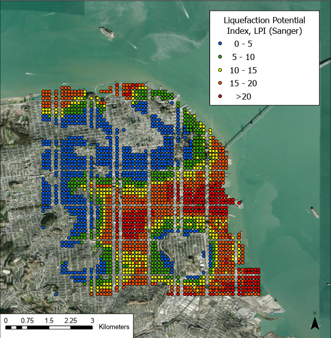
Fig 5. Results of the Sanger et al. (2024) model for liquefaction potential index given the selected M8 N. San Andreas rupture event scenario.
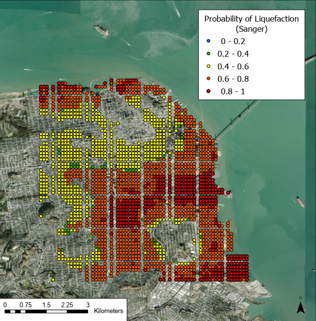
Fig 6. Results of the Sanger et al. (2024) model for probability of liquefaction given the selected M8 N. San Andreas rupture event scenario, using the Geyin and Maurer (2020) fragility function to map LPI to probability of surface manifestation (minor/all).
Remarks
Note
