The northern shore of Puerto Rico faces both seismic and oceanic hazards, making it an important area for tsunami hazard assessment. This example focuses on the town of Loíza and evaluates tsunami wave impacts using an integrated modeling workflow. Building inventories were developed with a Jupyter Notebook using BRAILS++, and a subsequent Notebook added 3D representations of these structures to bathymetric data obtained from NOAA. The combined datasets were formatted for use in Celeris, an open-source, interactive coastal wave simulation software that solves the extended Boussinesq equations. Celeris is integrated into the SimCenter HydroUQ toolset available on DesignSafe and was used to simulate tsunami inundation in Loíza under a specified scenario.
Tsunamis are powerful waves frequently initiated by earthquakes. Modeling tsunami inundation is vital for creating tsunami evacuation routes and for long term planning of mitigation efforts in coastal communities.
Tsunami risk analysis using R2D <https://simcenter.designsafe-ci.org/research-tools/hydro-uq/>_ relies on inundation depth and flow velocity as primary intensity measures. These parameters are typically obtained from simulation results in the form of raster files covering the study area. The raster data is then combined with a building inventory to extract the inundation depth and velocity at each structure. Accurate modeling of these intensity measures is critical for reliable loss estimation. Therefore, the simulation must account for wave-structure interactions, among other important factors not detailed here. Two widely adopted approaches exist for representing these interactions:
Equivalent Surface Roughness: This method uses roughness values to capture the effect of buildings and vegetation on propagation of water through a community. This method is advantageous due to its simplicity and compatibility with widely available digital elevation models, which generally attempt to remove buildings and vegetation.
Explicitly Represented Buildings: This method adds impermeable blocks to the digital elevation model corresponding to buildings. While real buildings do not behave as impermeable blocks during a tsunami, this method attempts to more directly model buildings’ effect on inundation. However, this method requires much higher resolution digital elevation models (and as a result, longer computing times) and an existing structural inventory.
A study by Sadashiva et al. [Sha22] compared these methods and determined models using explicitly represented buildings provided more realistic tsunami flow patterns and reduced uncertainly in loss calculations as compared to models using equivalent surface roughness.
While high resolution bathymetry and digital elevation models (DEMs) are becoming more available, many coastal communities like Loiza lack a complete structural inventory to be used in inundation modeling. Bridging this gap in available data is crucial for high accuracy inundation modeling and the associated risk and loss assessments.
Gathering and processing the data required for use with Celeris in this example occurs in three major steps:
Creation of Building Inventory
Existing building inventories for this region of Puerto Rico are sparse. In our study area, no buildings were found in the National Structure Inventory (NSI). To address this data gap, we used BRAILS++ (Building Recognition using Artificial Intelligence at Large Scale), an AI-enabled tool developed and maintained by the NHERI SimCenter. BRAILS++ employs machine learning models trained on satellite imagery to identify building footprint geometries and locations. It then applies neural networks trained on Google Street View images to estimate building attributes such as number of stories, roof shape, and construction material.BRAILS++ can be run through Python, and for this project, a Jupyter Notebook was developed to:
Define the boundaries of the study area,
Extract and save building footprint geometries using BRAILS++,
Integrate any available data from the NSI,
Retrieve Google Street View imagery for each building (when available), and
Apply BRAILS++ classifiers to estimate the number of floors for buildings with Street View coverage.
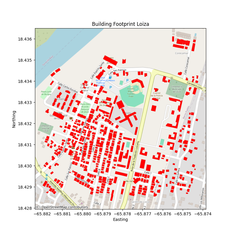
The following example uses BRAILS++ to create a building inventory for an approximately 800m by 800m area of Loiza, Puerto Rico. The area is centered at latitude 18.4323008 and longitude -65.8780065. The extent of the area is defined in degrees, with a radius of 400m in each direction.
Fig. 1. Building inventory of an approximately 800m by 800m area of Loiza, Puerto Rico.
Note
Number of floors is not estimated for buildings without StreetView data. As most of the buildings in this area are one floor, it is assumed that buildings with missing data are one floor.
Here is some example code that shows how an inventory can be created with BRAILS++:
1''' Install Brails++ ''' 2!pipinstallgit+https://github.com/NHERI-SimCenter/BrailsPlusPlus 3 4''' Import Packages ''' 5importnumpyasnp 6importpandasaspd 7frombrailsimportImporter 8 910''' Define an extent '''11lat=18.432300812long=-65.878006513r=400#m14# convert r from meters to ~degrees in lat and long15# Assumed constant circumferance of earth at 40075 km16r_lat=r*360/(40075*1000)17r_long=r*360/(40075*1000*np.cos(np.radians(lat)))1819lower_lat=lat-r_lat20lower_long=long-r_long2122upper_lat=lat+r_lat23upper_long=long+r_long2425extent=(lower_long,lower_lat,upper_long,upper_lat)2627''' Define a Brails++ Region Boundary Using the Extent '''28location=extent2930# Create an Importer instance:31importer=Importer()3233# region_data can also use location_name to define extent using:34# region_data = {"type": "locationName", "data": "Loiza, Puerto Rico"}35region_data={"type":"locationPolygon","data":extent}3637# Initialize the region boundary class and give it the region data38region_boundary_class=importer.get_class('RegionBoundary')39region_boundary_object=region_boundary_class(region_data)4041''' Generate Building Inventory '''42# Define footprint source:43# fpSource included in BRAILS are i) OpenStreetMaps,44# ii) Microsoft Global Building Footprints dataset, and iii) FEMA USA Structures.45# The keywords for these sources are OSM_FootprintScaper, MS_FootprintScaper,46# and USA_FootprintScaper, respectively.47footprint_scaper='OSM_FootprintScraper'4849# Initialize scaper class50scraper_class=importer.get_class(footprint_scaper)5152# define output units by passing to scraper class53lengthunit='m'# Options are 'm' or 'ft'54scraper=scraper_class({'length':lengthunit})5556# use get_footprints method to retreive footprints57footprints=scraper.get_footprints(region_boundary_object)5859# Check NSI database for exsisting stuctural data60# Initialize NSI Parser61nsi_class=importer.get_class('NSI_Parser')62nsi=nsi_class()6364# Run NSI Parser for the region boundary and combine with the footprints65nsi_inventory=nsi.get_filtered_data_given_inventory(66footprints,lengthunit)67_=nsi_inventory.write_to_geojson("LoizaBuildingInventory.geojson")
Note
Complete Jupyter notebook can be accessed in DesignSafe - Data Depot at PRJ-4604/Losses_Damage_R2D/BrailsPlusPlus_HJW/Loiza/ under the name InventoryBRAILS_Loiza.ipynb.
Gathering Existing Bathymetry/DEM:
Next, bathymetries with near-shore elevation data are required. The data used in this example is freely available through NOAA’s National Centers for Environmental Information at the Bathymetric Data Viewer website . From this website, data is downloaded as a raster file from the Continuously Updated DEM (CUDEM) dataset at resolution of 1/9 arc-second (~3m).
Fig. 2. Procedure to obtain DEM using the NOAA website.
The grid extract fuction allows for a box to be drawn by hand or for the extent to be specified with latitude and longitude. The extent of the DEM downloaded should provide a significant margin beyond the extent used to generate the building inventory.
Note
This data generation workflow can be applied to any coastal location with sufficiently fine DEM/bathymetry models, but larger areas slow the inventory creation time.
Combining Building Inventory With DEM:
At this stage of the process two important inputs have been gathered:
A DEM of the study area with an approximate resolution of 3m, and
A building inventory which contains footprint polygons and the estimated number of floors for each building.
A resolution of 3m is too large for explicitly modeled buildings. Buildings will appear overly pixelated when added to a 3m DEM. To overcome this issue the DEM is upsampled by a factor of 2, to a resolution of ~1.5m.
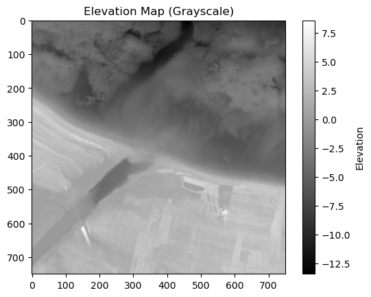
Fig. 3. Unaltered DEM of Loiza coastline plotted by pixel.
The building inventory is then rasterized to a matching resolution of 1.5m. In this step it is assumed that story heights are equal to 3m. The outcome is a DEM in which all points within the footprint of a building are set to the elevation of the roof height, and all other points are set to an elevation of zero.
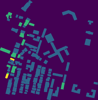
Fig. 4. Rasterized building inventory from a approximately 400m by 400m region of Loiza.
With the building inventory and DEM in compatible formats they can be added together and formatted to be compatible with Celeris.
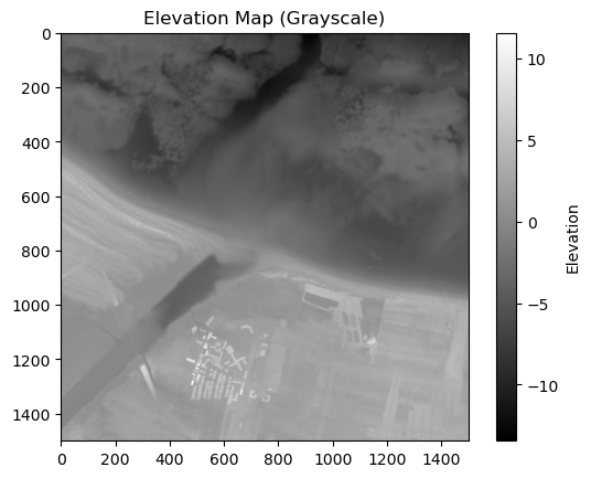
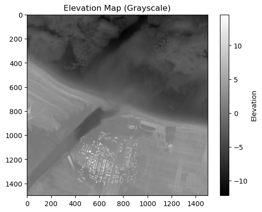
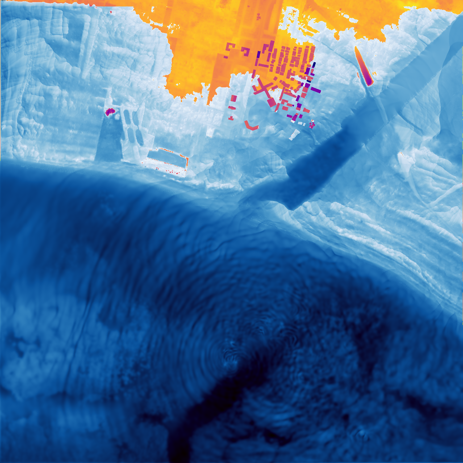
Fig. 5 (a). Combined DEM and building inventory from a 400m by 400m region of Loiza.
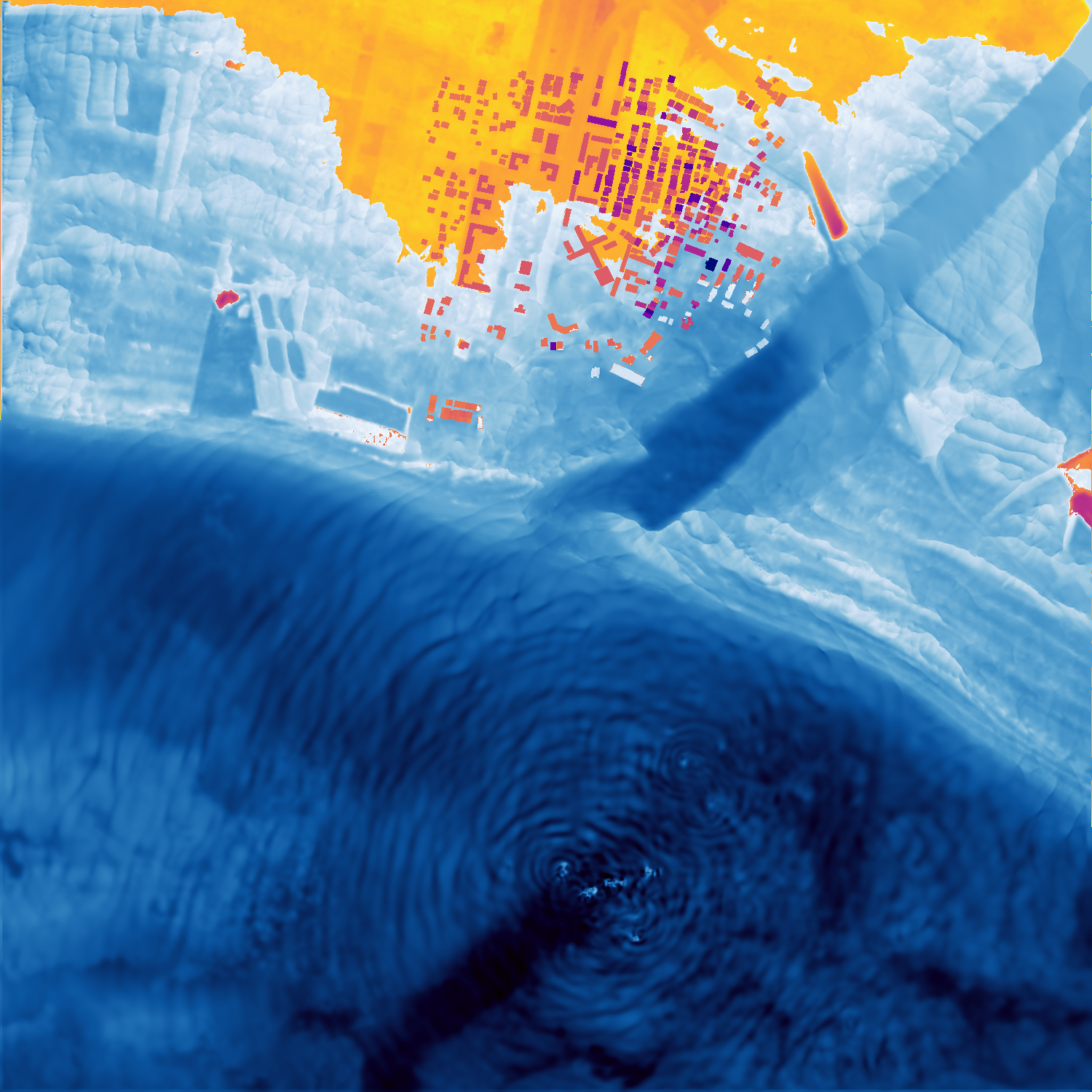
Fig. 5 (b). Combined DEM and building inventory from a 800m by 800m region of Loiza.
Note
Inventory combination was implemented in a Jupyter Notebook that can be accessed in DesignSafe - Data Depot at PRJ-3948/HydroUQ/Celeris/notebooks/ under the name CombinedBathymetry.ipynb. Current implementation requires manually aligning the inventory and DEM using an arbitrary offset.
Download the Celeris file (from above or from the SimCenter BackEndApplications) and place it on a computer with a GPU (e.g. on a Frontera rtx-dev allocation accessed through DesignSafe). Be sure the computer can also run a version of Python compatible with Taichi, a Python package that allows for the use of a GPU to perfrom parallel computations.
Note
Downloading Celeris from SimCenterBackendApplications on GitHub will not have the Loiza example. To run this example, download the relevant files here:
Place the file inside SimCenterBackendApplications at SimCenterBackendApplications\modules\createEVENT\Celeris\examples.
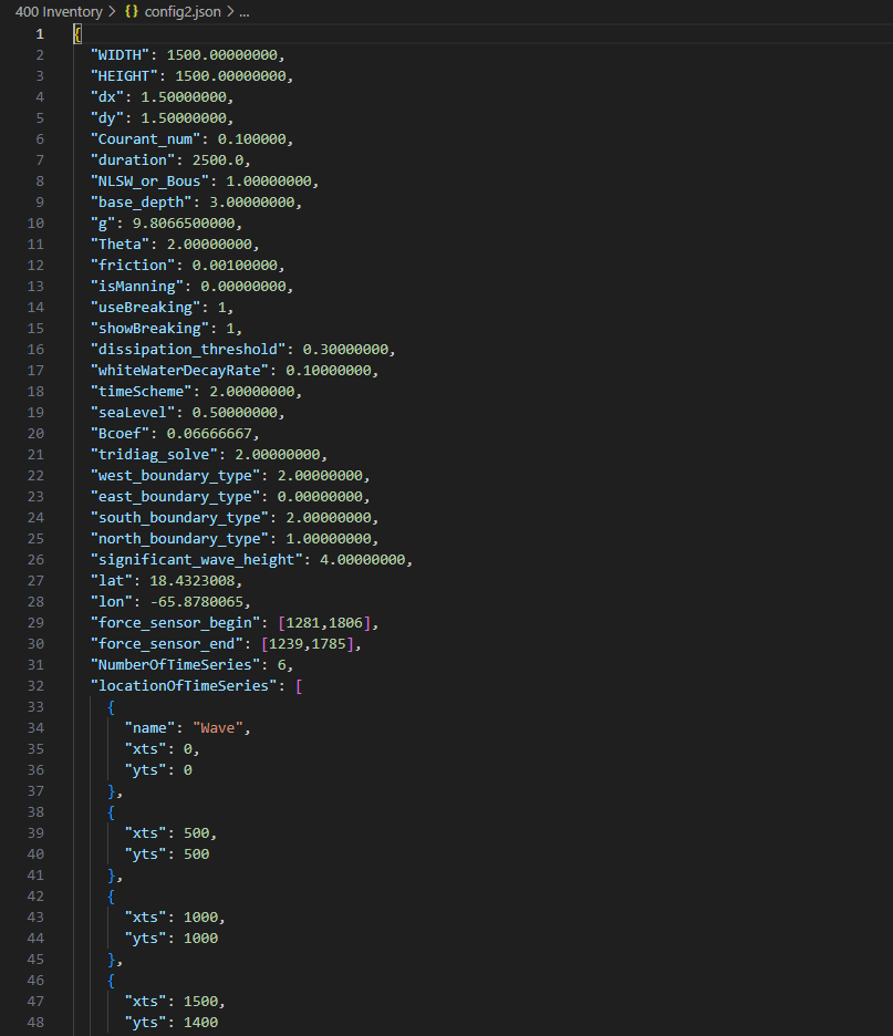
Files defining bathymetries, waves, and other settings can be found at Celeris\examples\Loiza. The files containing the bathymetries generated are stored here as bathy2.txt and bathy4.txt for the 400m by 400m and the 800m by 800m inventories respectively. The file, wave.txt, was used for both bathymetries. The configuration (config2.json and config4.json) files contain the general settings required to run the model including the DEM resolution as “dx” and “dy”. Simulated wave gauges and a force sensor were placed at locations of interest in Loiza and are defined here under “locationOfTimeSeries”, and “force_sensor_begin” and “force_sensor_end”.
wave.txt is a default wave file and has not been modified. To obtain meaningful results, a wave file from known historic wave heights and velocities should be used. If this data is unavailable, tsunami propagation to the near shore should be simulated using an associated probabilistic seismic event. See [Sha22] and [Gri15] for more on tsunami source and propagation modeling.
Note
There are several other import settings in the configuration files not described in detail here.
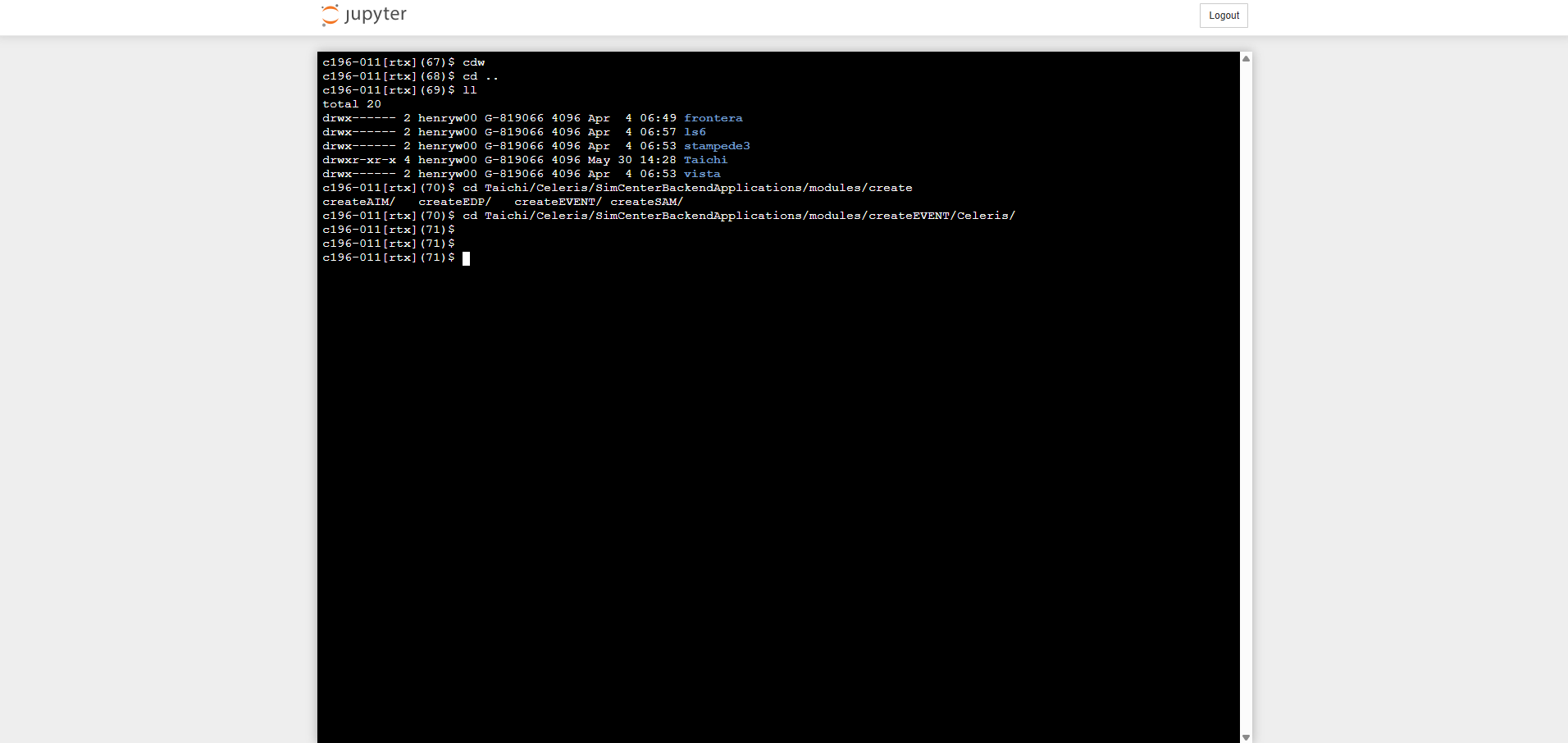
With all the proper files in place, Celeris can be run from the terminal. To do this, open a terminal and navigate to the Celeris folder.
For this example, Celeris is running in a rtx-dev frontera allocation through DesignSafe.
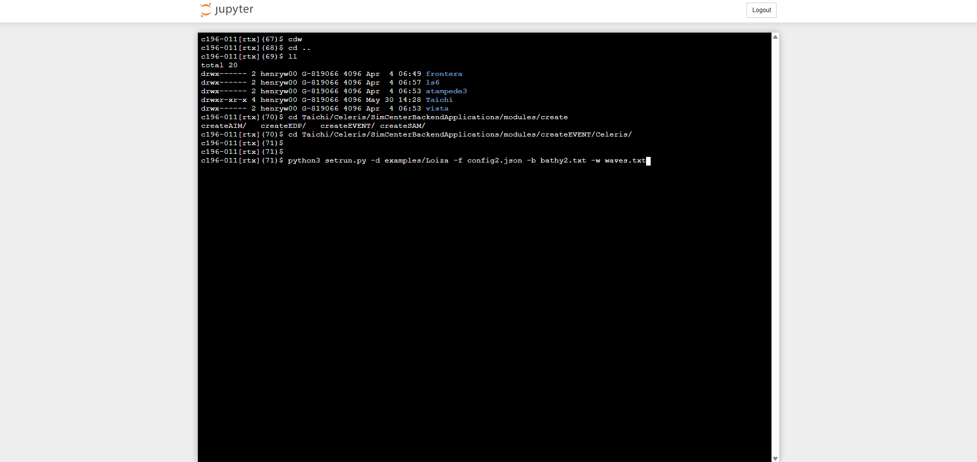
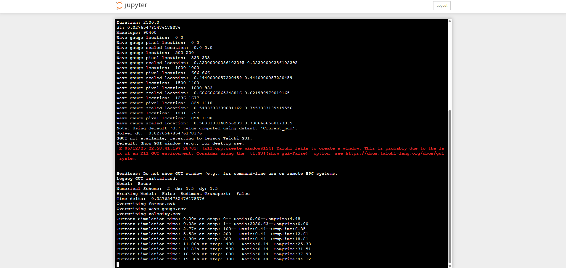
Run the command: python3setrun.py-dexamples/Loiza-fconfig2.json-bbathy2.txt-wwaves.txt. This simulates the inundation of the 400m by 400m inventory. To simulate the inundation of the 800m by 800m inventory, instead use the input files, bathy4.txt and config4.json.
After Celeris finishes running, results will be saved in the Celeris folder.
Still images from the simulation and a .gif animation will be saved to Celeris/plots. Depth and velocity data at each of the wave gauges will be saved to Celeris/wave_gauge.csv and Celeris/velocity.csv. Force data will be saved to Celeris/forces.csv.
Fig. 10 (a). A frame from the simulation for the 400m by 400m inventory.
Fig. 10 (b). A frame from the simulation for the 800m by 800m inventory.
In the animations it can be seen that most of the flooding does not result from water running up the beach. Instead it occurs as water flows up the river and overtops the banks.
Links to the full simulation animations are available here:
With the current method for formatting bathymetries for Celeris, the bathymetry is rotated 180 degrees, meaning north is down for these results.
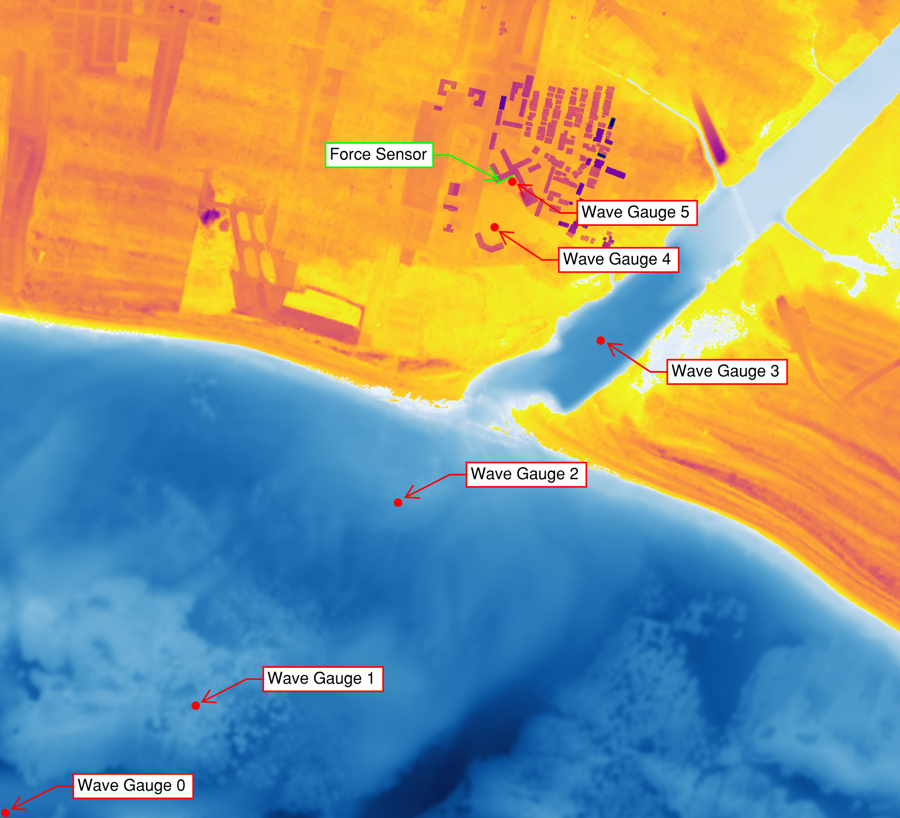
For this example, six wave gauges and one force sensor were placed at various locations throughout the study area. Three wave gages were placed offshore (wave gauges 0 through 2), one was placed in the nearby river (wave gauge 3), one was placed in school’s baseball field (wave gauge 4), and one was placed adjacent to the school (wave gauge 5). The force sensor was placed along one of the wings of the school. Gauge and sensor locations for both the 400m by 400m simulation and the 800m by 800m simulation are in approximately the same location (except for wave gauge 0 which had to be adjusted due to slight differances in the bathymetry boundaries).
Wave gauges in Celeris measure both water depth and velocity, and the force sensor measures various components of force. The results of each are presented here:
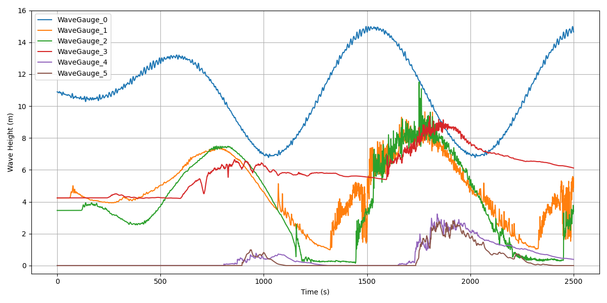
Water Depth:
Fig. 12 (a). 400m by 400m water depth time series.
Fig. 12 (b). 800m by 800m water depth time series.
Generally, the depth time series from the 400m and 800m cases match well. There are some minor differences in the noise of each. There is one major difference. At wave gauge 0 the depth in the 400m case is consistently ~1m greater than the 800m case. This difference is a result of the slight offset of the location of wave gauge 0 between the scenarios.
In both cases wave gauge 0 provides a generally unaltered view of the incoming wave. Wave gauges 1, 2, and 3 show how the wave height changes as it approaches the shore and propagates up the river. Wave gauges 4 and 5 show the level of inundation nearby and adjacent to the school.
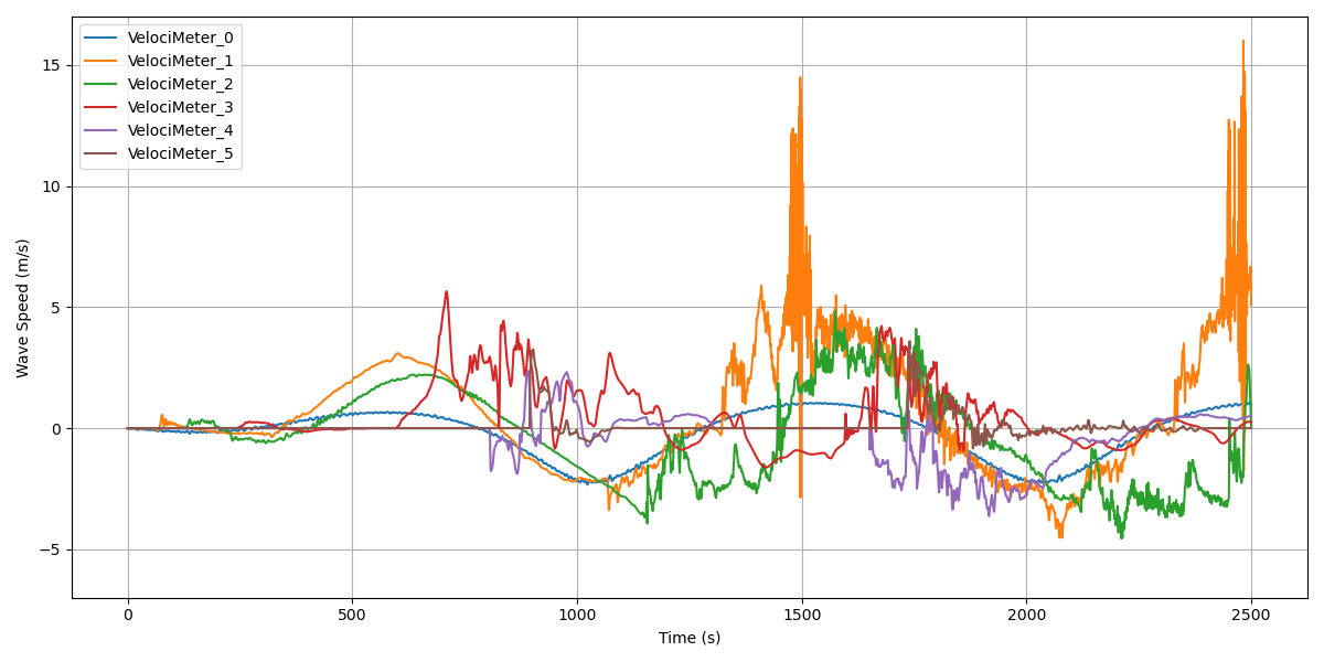
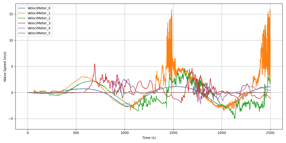
Like the depth results, the velocity time series are similar in both simulations with only one notable difference. The velocity at wave gauge 4 in the 400m by 400m case reverses earlier and for longer than in the 800m by 800m case. This may only be a difference in noise, but in rewatching the 400m animation there is a pulse of water that floods the baseball field, which is not present in the 800m animation. It is possible that this difference results from additional buildings dispersing this pulse before it reaches the baseball field.
Forces:
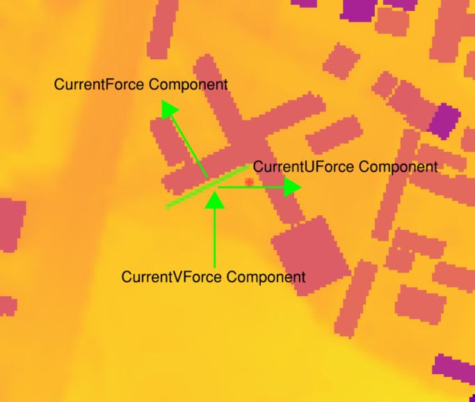
In Celeris, forces are calculated as 4 different components:
CurrentUForce: This component of hydrodynamic force acts horizontally with respect to the bathymetry’s coordinate system (i.e. in the east/west direction).
CurrentVForce: This component of hydrodynamic force acts vertically with respect to the bathymetry’s coordinate system (i.e. in the north/south direction).
CurrentForce: This component of hydrodynamic force acts in the direction of the normal vector of the force sensor. It is positive when the force is opposed to the normal vector and zero otherwise (i.e. the water is retreating).
HydrostaticForce: This is the component of force associated with the hydrostatic pressure on the sensor. It acts parallel to CurrentForce.
Fig. 14. A diagram of the hydrodynamic force components.
Note
Hydrodynamic forces are calculated assuming all fluid momentum is stopped by a wall parallel to the force sensor. Therefore, the force data is only meaningful when the force sensor is placed along the wall of a building that is not overtopped.
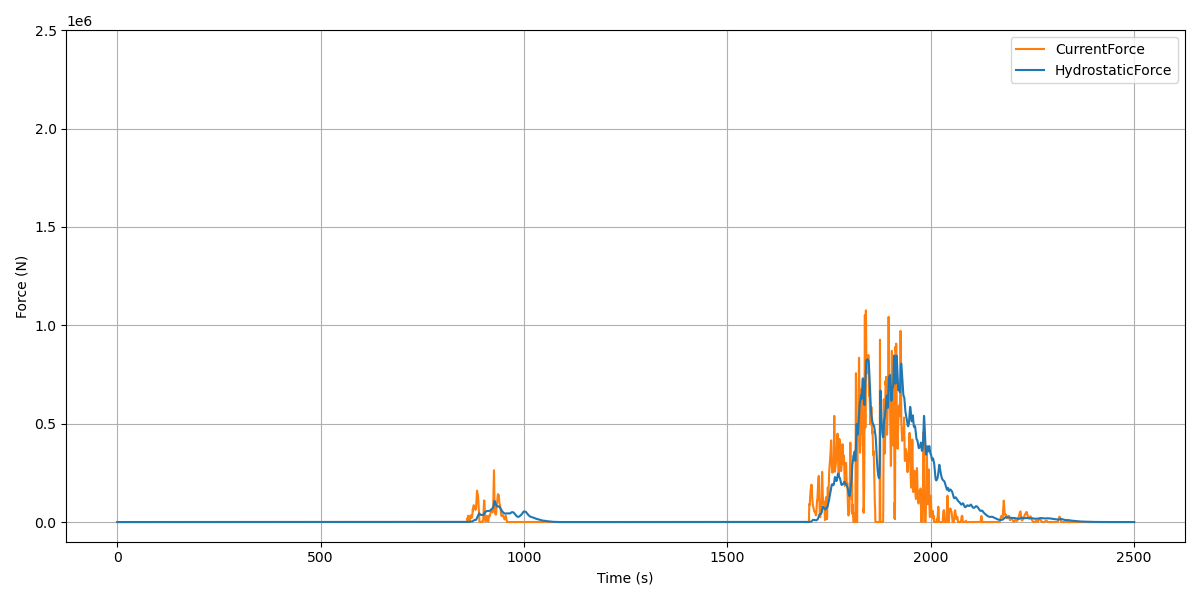
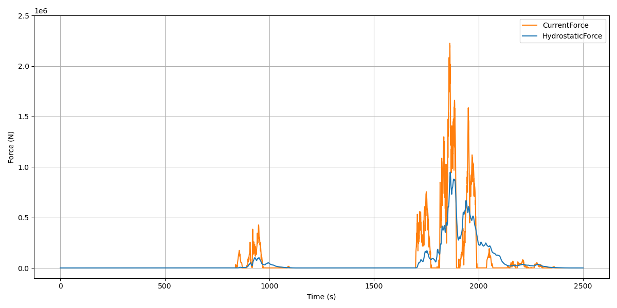
For simplicity, only HydrostaticForce and CurrentForce are plotted.
The hydrostatic force in each scenario likely only differs due to noise. In contrast, the peak CurrentForce in the 800m scenario is more than double the peak CurrentForce in the 400m scenario. It seems likely that the additional buildings between the river shore and school act to concentrate flow, increasing the current force on the sensor.
Warning
All results presented here use a hypothetical wave and are therefore hypothetical. Any conclusion drawn from them should also be treated as such.
For reliable results, use many waves with many associated seismic triggers. Sensitivity testing should be performed on each model input, including inventory size and bathymetry resolution.
