R2D - Landslides
Introduction
This page describes a preliminarly approach for landslide risk assesment which propose an initial workflow that must be developed in the future, so then it can implemented in the SimCenter tool R2D. An example, which uses Jibson (1993) model to predict Newmark sliding block displacements, is presented for a portion of the city of Seattle, WA. Resources from SimCenter M9 project are used in the example to estimate ground-motion intensity parameters.
Problem Description
Studying earthquake-induced landslides is vital for reducing risks, protecting lives and property, preserving the environment, and enhancing our scientific understanding of these natural disasters. Through comprehensive research and application of findings, societies can better prepare for and mitigate the impacts of these potentially devastating events.
There are several models that can be implemented in a regional-based study so that, hazard values it can be estimated. Some researchers use the theory of Newmark Sliding Block [New65] to predict how much displacement would occur if an earthquake with a certain ground motion were to occurr. These models have developed correlations that depend on different intensity measurements as: Earthquake Magnitude (\(M_w\)), Peak Ground Acceleration (\(PGA\)), Peak Ground Velocity (\(PGV\)), Arias Intensity (\(I_a\)), Critical Acceleration (\(a_c\)), Normalized Critical Acceleration (\(k_c\)), Spectral Acceleration (\(Sa\)), Static Factor of Safety (\(FS_{static}\)), and Ground Sloping (\(\beta\)), as well as Soil Strength Parameters (\(\gamma,\:c,\:\phi\)).
This models could be built-in within R2D tool so that we can estimate Damage and Losses against earthquake-induced landslides.
Solution Strategy
In this section, we propose a preliminarly workflow that can be coded within R2D so we can estimate damage and losses as consequences of earthquake-induced landslides risk.
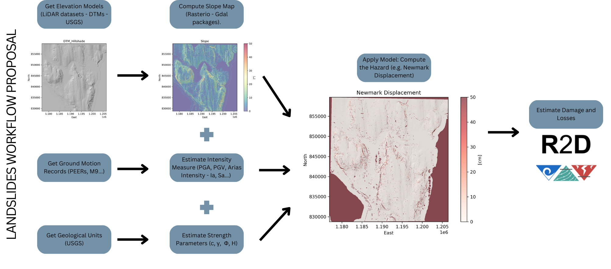
Figure 1. Proposed workflow for incorporating Landslide Risk Assesment into R2D.
Here are some steps to consider:
Same as the BRAILS tool is embedded within R2D we would need to embed a tool that allows the user to get Digital Elevation Models (DEM) from publicaly available GIS services (e.g. USGS portal). newline Then, a slope raster can be generated for the selected area (geospatial packages must be installed in python dependencies: Gdal, Rasterio).
Intensity measurements can be estimated from the “Earthqueake Event Generation” tool. Reminder that some of the models use mesurements extracted from the time-history record, whereas others use spectral accelerations (extracted from the reponse spectrum).
Soil Strength Parameters can be estimated from geological mapping and reference values correlations. So, a tool that allows the user to get geological GIS units must be built-in within R2D as well.
Finally, after input parameters can be estimated for a certain model, the hazard values can be calculated as Newmark Displacement values.
Note
All of the previous estimations have uncertainty and the model itself has its own uncertainty.
SimCenter Tool Used
The goal is to implement the following protocol into R2D. However some Simcenter tools were used in order to develop the procedure.
The Simcenter Jupyter HUB was used to write the notebook that would help us to compute the hazard against landslide.
Ground motions from SimCenter project M9 were used as a grid to which then, intensity measurements would be calculated.
Example Application
In this section we would like to analyze in a regional scale, what would be the response across a study area located in Seattle, WA, US. The idea is to estimate the predicted displacement in the study area if an earthquake with certain intensity measure (Arias Intensity \(I_a\)) were to occur. The model integrates the infinite slope approach to estimate the static factor of safety so then the Critical Acceleration \(a_c\) can be estimated. Finally with these parameters a Newmark displacement could be estimated using Randall W. Jibson correlation [Jib93]:
Where:
\(Dn\) = Newmark Displacement [cm].
\(I_a\) = Areas Intensity [m/s].
\(a_c\) = Critical Acceleration [g].
Also,
Where:
\(\beta\) = Slope Angle [°].
\(FS_{static}\) = Static Factor of Safety [-].
\(c\) = Cohesion [kPa].
\(\gamma\) = Unit Weight [kN/m³].
\(\phi\) = Friction Angle [°].
\(I_a\) = Intensity measure time-history motion specific.
A Jupyter Notebook has been developed to code the implementation of the previous model in the area of interest:
- Get the Digital Elevation Model for the area of interest and perform the slope calculations: The USGS portal is used to download the LiDAR data in the area of interest. See Figure 2 to check the area of interest.
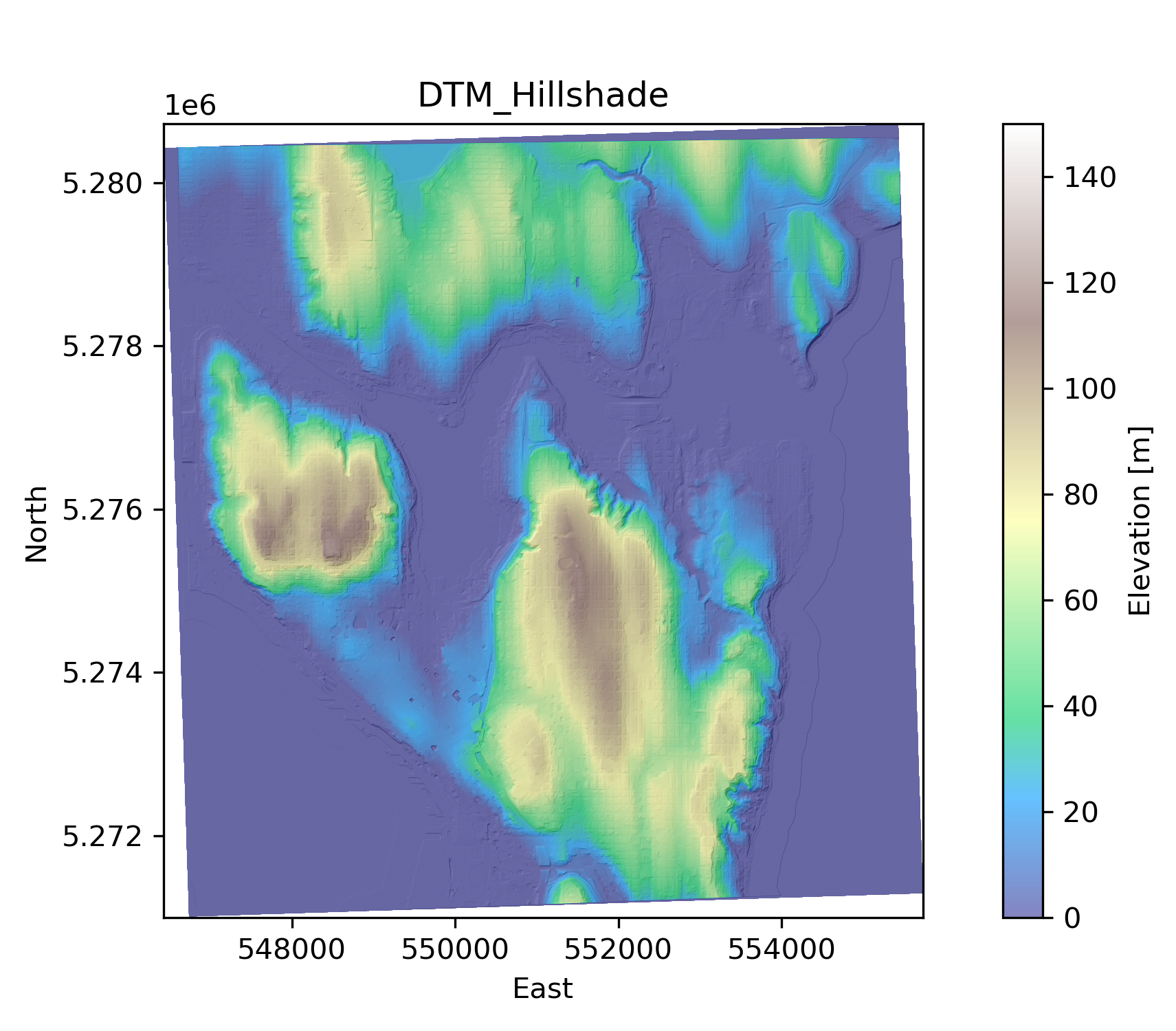
Figure 2. Raster DTM - downloaded from the USGS GIS Service.
Subsequently the Slope map is calculated using the Gdal library. See Figure 3 to check the slope map in the area of interest, Seattle WA.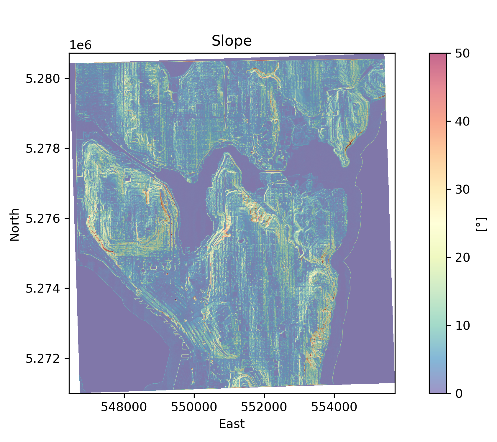
Figure 3. Raster Slope - computed with GDAL.
- Get the Intensity Measurements: The intensity values (Areas Intensity in this example) are computed using motions from the M9 project which is a suite of synthetic ground motions for a range of possible magnitude 9 earthquake rupture scenarios on the Cascadia megathrust.
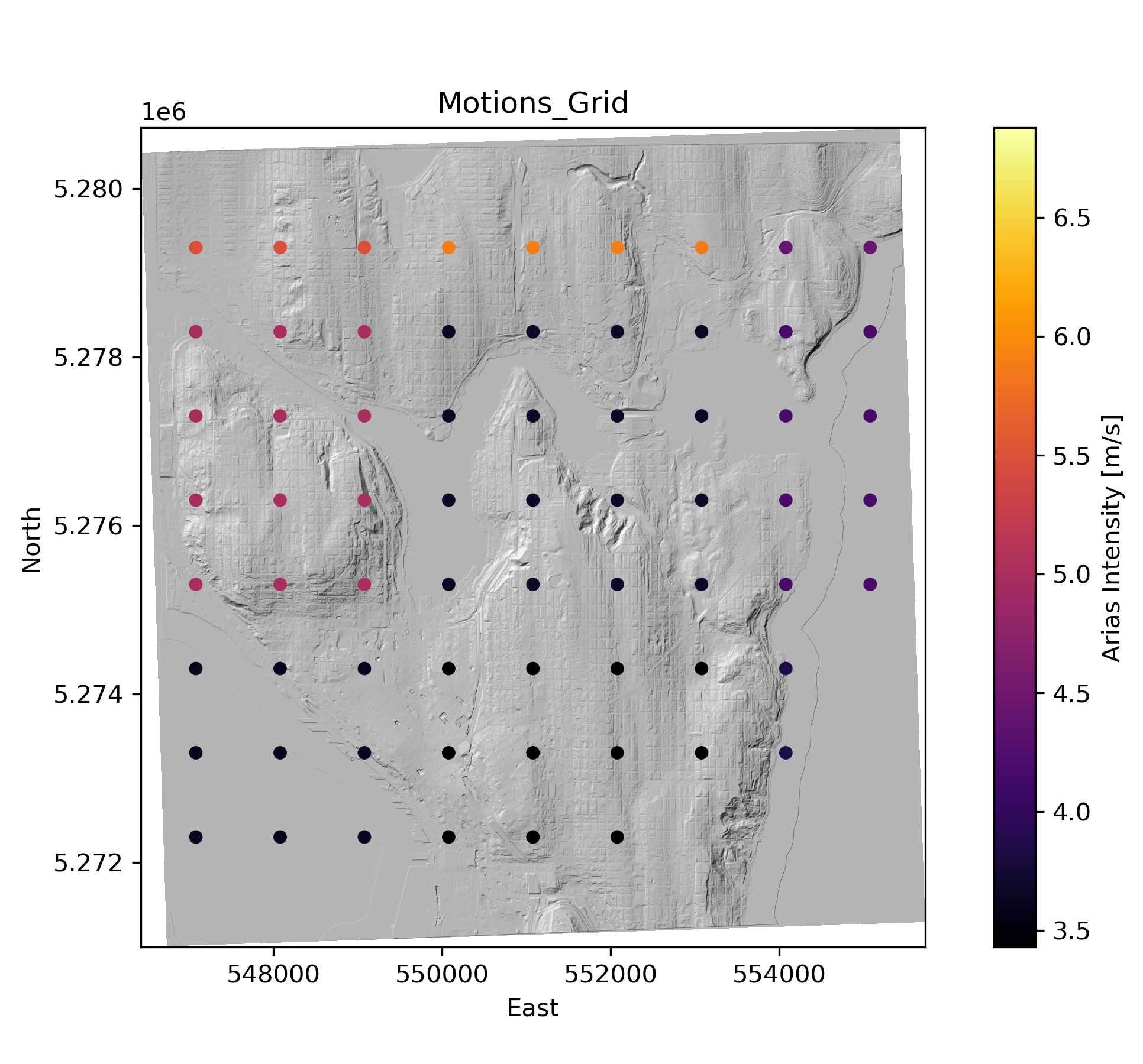
Figure 4. Motions Grid - Legend indicates values of Arias Intensity [m/s].
The value of areas intensity will be given by the nearest neighbor motion in the grid. A raster with intensity measures is created from the grids. Figure 5 is an example of how the Arias intensity would look like after applying the nearest neighbor method. Most of this work is done using the package Rasterio.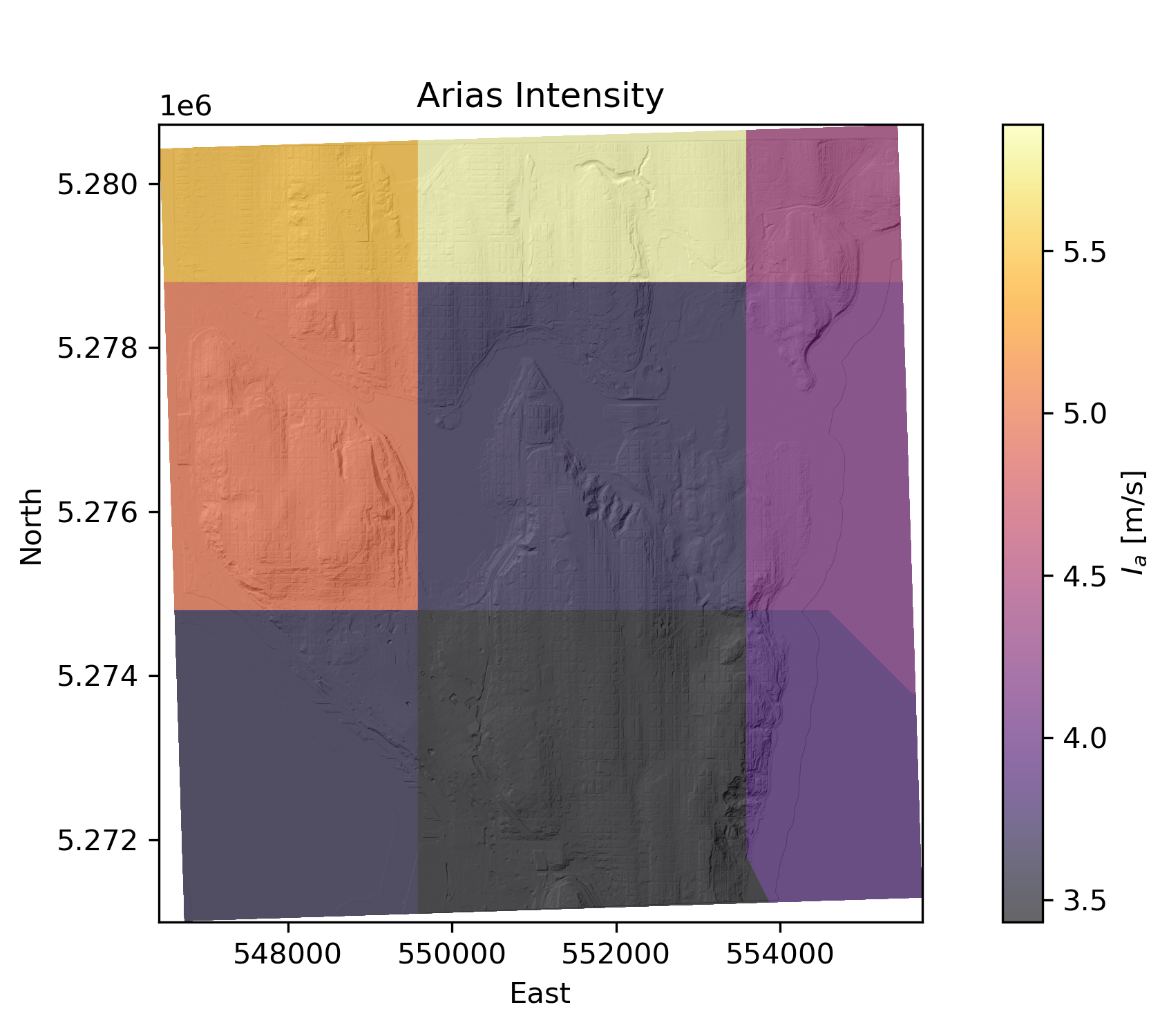
Figure 5. Interpolation using Nearest Neighbor for Arias Intensity [m/s] values.
Warning
Either Rasters and Motions should be self-consistent with a single spatial reference.
- Get the Soil Stregth Parameters: as it is for now, this measurement can be heuristically set by the user while the code is built.
Finally, when all the inputs variables are estimated, we can implement the Randall W. Jibson model in the study area. Figure 4 displays the calculated Newmark Displacement for our area of interest Seattle.
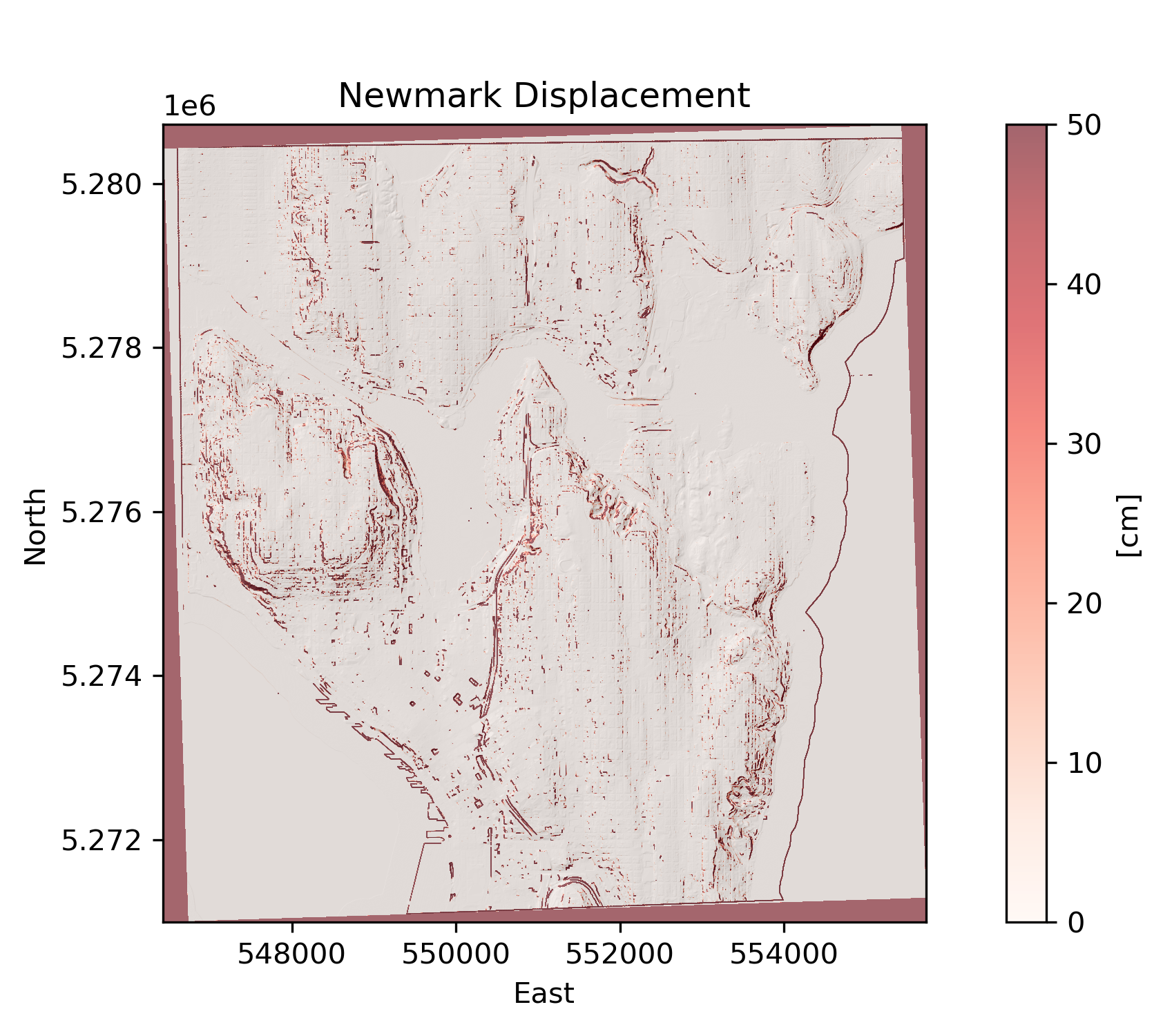
Figure 6. Randall W. Jibson calculated Newmark Displacement.
Remarks
A Jupyter Notebook (‘hazardNewmark.ipynb’) was coded to simulate the process that could be implemented to R2D for earthquake-induced landslides hazard so the user could then estimate damage and losses. Please if refering to this notebook, careful read the instructions in the readme first. Find this work in the CESG599 repository. When trying to run this notebook, you must have access to the M9 project in DesignSafe machines.
Earthquake induced landslides prediction may be a difficult task to adress, but there are models out there that can be implemented to predict the hazard and subsequently, this hazard can be used to predict damage amd losses. The idea is in this section is to provide a procedure that could ve developed within the SiimCenter R2D tool to predict the hazard and subsequently, to predict damage amd losses.